Chapter 17 ANOVA Part 2: Partitioning Sums of Squares
The 1-Factor ANOVA compares means across at least two groups. In the last chapter we discussed the intuition that ANOVA is about comparing the variances between the means across the groups to the mean of the variances within each group. While this intuition is useful, it’s not a practical way to calculate F-statistics from your data, mostly because it doesn’t deal with differences in sample sizes between groups, and doesn’t help to understand more complicated experimental designs.
This chapter covers the more traditional way to explain ANOVA, which is in terms of breaking down sums-of-squared deviations from means. This was the most popular way to think about ANOVA for years until recently when we’ve moved toward regression as a framework for ANOVA. But the sums-of-squares framework is useful because it shows you how ANOVA is computed “by hand,” and it generalizes cleanly to more complicated designs. Later we’ll see that regression gives the same results, but from a different point of view.
In this chapter we’ll define the formulas for calculating the numerator and denominators of the F-statistic and then go through the calculations in R. You can guess that R has it’s own function for running ANOVAs, which we’ll do at the end to check that we have the right answers.
We’ll work with an example from the survey. I’ve always had the intuition that students in the front are more ambitious and engaged, so perhaps they are doing better in school compared to the students that sit in the middle or back of the class. Let’s go to the survey data again and see if there is a difference in the student’s GPA at UW when we divide the class into groups based on where they like to sit in the classroom.
The variable we take means of is the dependent variable (a continuous outcome), which is UW GPA in this example. The variable we use to form groups is the independent variable. In ANOVA, this is a nominal variable called a factor. The different options of a factor are called its levels.
Here’s some code that generates a summary table based on the survey data. It uses tapply to calculate means, sums and standard deviations across the three levels of our factor. The slightly weird part is the call to the function factor which determines the order of the levels in our factor. By default, R puts things in alphabetical order, and we want to choose the order ourselves: front > middle > back
survey <-read.csv("http://www.courses.washington.edu/psy315/datasets/Psych315W21survey.csv")

survey$sit <- factor(survey$sit,levels = c(
  "Near the front", "In the middle", "Toward the back"), ordered = TRUE)

# define our statistics here - we'll be using them later.
ns <- tapply(survey$GPA_UW,survey$sit,function(x) sum(!is.na(x)))
means <- tapply(survey$GPA_UW,survey$sit,mean,na.rm = TRUE)
sds <- tapply(survey$GPA_UW,survey$sit,sd,na.rm = TRUE)
sems <- sds/sqrt(ns)

# stick them into a data frame for plotting
summary <- data.frame(n=ns,mean=means,sd=sds,sem=sems)| n | mean | sd | sem | |
|---|---|---|---|---|
| Near the front | 47 | 3.54 | 0.34 | 0.05 |
| In the middle | 71 | 3.51 | 0.30 | 0.04 |
| Toward the back | 32 | 3.35 | 0.43 | 0.08 |
The means do differ, but it’s hard to see by how much compared to the standard errors. Let’s use this table to make a bar plot of the means with error bars set to \(\pm\) one standard error of the mean:
# Define y limits for the bar graph
ylimit <-  c(min(summary$mean-1.5*summary$sem),
             max(summary$mean+1.5*summary$sem))

# Plot bar graph with error bar as one standard error (standard error of the mean/SEM)
p <- ggplot(summary, aes(x = row.names(summary), y = mean)) +
  xlab("Where do you like to sit in class?") +
  geom_col(position = position_dodge(), color = "black", fill="lightblue")

p+geom_errorbar(aes(ymin=mean-sem, ymax=mean+sem),width = .5) +
  scale_y_continuous(name = "GPA at UW") +
  scale_x_discrete(limits = row.names(summary)) +
  coord_cartesian(ylim=ylimit) + theme_bw()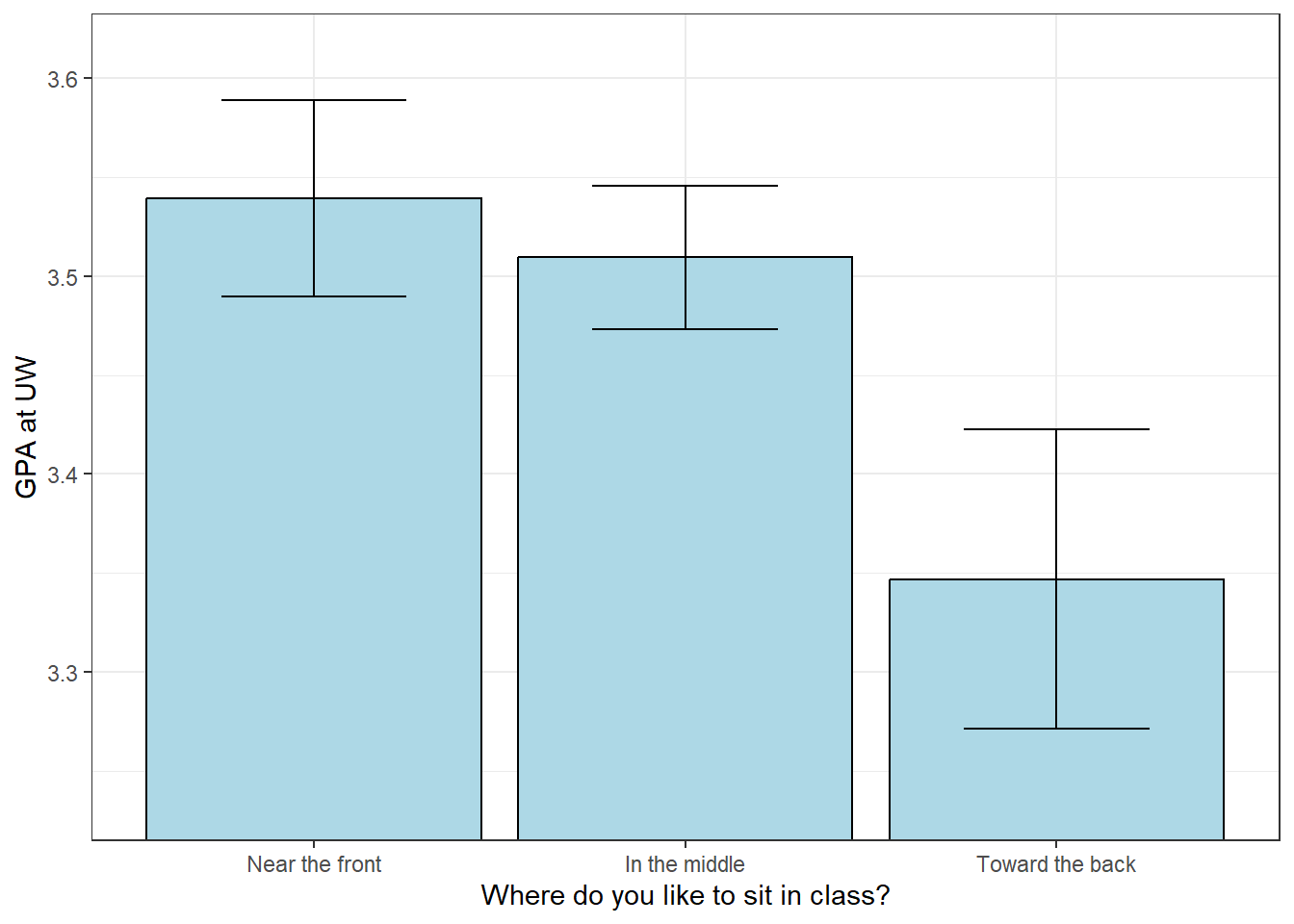
Remember the rule of thumb for the two-sample independent measures t-test: you need a gap in the error bars for a statistically significant difference. We use the same rule here to compare two means a time.
17.1 Familywise error
You might think that we could just run a bunch of independent measures t-tests to see which pairs of mean are significantly different. The problem is the issue of ‘multiple comparisons’. If the null hypothesis is true and all three means are drawn from populations with the same mean, then the probability of rejecting any test is \(\alpha\). But if there are multiple tests, the probability of rejecting one or more of these tests becomes greater than \(\alpha\)
If there are k levels, then there are \(m = \frac{k(k-1)}{2}\) possible pairs. There are m = 3 pairs for our three-level example. If \(H_{0}\) is true, then the probability of failing to reject any test is \(1-\alpha\). With m tests, the probability of failing to reject all of them (if they’re independent) is \((1-\alpha)^{m}\). So the probability of rejecting one or more is the opposite of failing rejecting all of them: \(1-(1-\alpha)^{m}\)
For our example, if we let \(\alpha = 0.05\):
\[1-(1-\alpha)^{m} = 1-(1-0.05)^{3} = 0.1426\]
This is much higher than \(\alpha\) = 0.05. This means that if \(H_{0}\) is true and we run all possible hypothesis tests, we’ll make one or more type I errors about 14 percent of the time. This probability grows quickly with the number of levels. For an experiment with 10 levels,
\[1-(1-\alpha)^{m} = 1-(1-0.05)^{10} = 0.4013\] If we only report the significant outcomes, you can see how Type I errors creep in to the literature.
Technically this math isn’t quite right because these tests aren’t statistically independent. The chapter on Apriori and Post-Hoc Comparisons goes into excruciating detail about ways to deal with this issue of familywise error if we do want to make multiple hypothesis tests.
ANOVA is way of comparing all of the means to each other with one test, thereby avoiding familywise error. The drawback is that if there is a significant difference between the means, the test doesn’t tell you how they are different. They all could be a little different from each other, or one of the means could be very different from the others.
17.2 Partitioning Sums of Squares
Back to our example. If we call our dependent measure \(X\), let \(X_{ij}\) be the i th data point in level j. Let k be the number of levels, so j will range 1 to k. Let \(n_{j}\) be the sample size for level j, so i will range from 1 to \(n_{j}\).
Let \(\overline{X}_{j}\) be the mean for level j, and let \(\overline{\overline{X}}\) be the grand mean, which is the mean of the entire data set. Note, despite it’s symbol, \(\overline{\overline{X}}\) will not necessarily be equal to the mean of the means unless the sample sizes are equal.
Consider the plot below which shows a bar graph of our survey data, but with each data point shown individually. I’ve highlighted a few values. First, I’ve picked out a single data point, \(X_{ij}\) which I’ve shown in \(\color{red}{\text{red}}\). The mean of the level that it came from, \(\overline{X}_{j}\) is colored in \(\color{green}{\text{green}}\), and the grand mean, \(\overline{\overline{X}}\) I’ve shown in is colored in \(\color{blue}{\text{blue}}\)

Consider how far our chosen data point is away from the grand mean: \(X_{ij}-\overline{\overline{X}}\). We can separate this difference, or deviation into two parts:
\[ (X_{ij}-\overline{\overline{X}}) = (X_{ij} - \overline{X}_{j}) + (\overline{X}_{j} -\overline{\overline{X}})\] This is not advanced algebra, but it illustrates the point that the deviation between any data point and the grand mean is the sum of the deviation between that point and the level’s mean and the deviation between the level’s mean and the grand mean. Where were going is that the term \((X_{ij} - \overline{X}_{j})\) contributes to the mean of the variances within each level, and \((\overline{X}_{j} -\overline{\overline{X}})\) contributes to variance of the means between the levels.
While the above equation is trivially true, the following equation is also true:
\[ \sum_{j=1}^{k}\sum_{i=1}^{n_{j}}{{(X_{ij}-\overline{\overline{X}})^{2}}}= \sum_{j=1}^{k}\sum_{i=1}^{n_{j}}{(X_{ij} - \overline{X}_{j})^{2}} + \sum_{j=1}^{k}\sum_{i=1}^{n_{j}}{(\overline{X}_{j} -\overline{\overline{X}})^{2}}\] The double sums means that we’re summing across the entire data set by first summing across the samples within each level, and then summing that sum across the levels.
You can’t normally just square terms on both sides of an equation and add them up, but it turns out that it works for this special case with means. Specifically, because the within-group deviations sum to zero within each group, the cross-term cancels when you expand the square. Each of these three terms are called ‘sums of squares’ or SS, and each has it’s own name and meaning.
The first term is called sums of squares total. We can be sloppy and drop the double sum, assuming that we’re summing across the whole data set. It is written as:
\[SS_{total} =\sum_{ij}{(X_{ij}-\overline{\overline{X}})^{2}}\].
The second term is called sums of squared_within, written as:
\[SS_{within} =\sum_{ij}{(X_{ij} - \overline{X}_{j})^{2}}\].
It’s called within because it’s the sum of squared of the deviations of the mean within each level.
The last term is called sums of squared between. If you look at the inner sum, it’s the sum of \(n_{j}\) values of the same thing, so for each level, \(\sum_{i=1}^{n_{j}}{(\overline{X}_{j} -\overline{\overline{X}})^{2}} = n_{j}(\overline{X}_{j} -\overline{\overline{X}})^{2}\)
sums of squared between can therefore be written as:
\[ SS_{between} = \sum_{j} n_{j}(\overline{X}_{j} -\overline{\overline{X}})^{2} \]
It’s called between because it’s the sums of squared of the means between the levels (multiplied by the sample size).
Using the formula above:
\[ SS_{total} = SS_{within} + SS_{between}\]
Remember in the last chapter, where we discussed ANOVA as the ratio of the variance between groups and the variance within each group. The between partition is a measure of the variability across the means, which will be part of the numerator of the F-statistic. The within partition is a measure of the variability within each level and will contribute to the denominator of the F-statistic.
All we need to do is divide each of these sums of squares by their degrees of freedom and we can get variances. In the context of ANOVA, variance is called ‘mean squared error’, or MS, since it’s (sort of) the mean of the sums of squared deviation.
If N is the total sample size (\(\sum{n_j}\)), then the total variance, which we call mean squares total is:
\[MS_{total} =\frac{\sum{(X_{ij}-\overline{\overline{X}})^{2}}}{N-1}\].
For the within partition, each mean contributes \(n_{j}-1\) degrees of freedom, so the degrees of freedom added across all k levels is \(\sum{n_{j}-1}\) = \(N-k\). mean squares within is therefore:
\[MS_{within} = \frac{\sum{(X_{ij} - \overline{X}_{j})^{2}}}{N-k}\] If the sample sizes are equal then the above equation simplifies to the mean of the variances within each group, which you might recognize this from the last chapter.
For the between partition, it’s the variance of only k means, so the degrees of freedom is k-1. \(MS_{between}\) is written as:
\[ MS_{between} = \frac{\sum n_{j}(\overline{X}_{j} -\overline{\overline{X}})^{2}}{k-1} \]
You might recognize that this from the last chapter as the variance of the means multiplied by the sample size, except that this formula allows for different sample sizes.
17.2.1 Calculating F
The F-statistic is the ratio of \(MS_{between}\) and \(MS_{within}\):
\[ F = \frac{SS_{between}/(k-1)}{SS_{within}/(N-k)} =\frac{MS_{between}}{MS_{within}} \]
and the degrees of freedom are \(k-1\) and \(N-k\).
Notice that just like the sums of squares, the degrees of freedom also add up:
\[df_{total} = df_{within} + df_{between}\]
\[ N -1= (N-k) + (k-1)\]
It’s convenient to write all of this in a summary table like this:
| df | SS | MS | F | |
|---|---|---|---|---|
| Between | \(k-1\) | \(\sum_{j} n_{j}(\overline{X}_{j} -\overline{\overline{X}})^{2}\) | \(\frac{SS_{between}}{df_{between}}\) | \(\frac{MS_{between}}{MS_{within}}\) |
| Within | \(N-k\) | \(\sum_{ij}{(X_{ij} - \overline{X}_{j})^{2}}\) | \(\frac{SS_{within}}{df_{within}}\) | |
| Total | \(N-1\) | \(\sum_{ij}{(X_{ij}-\overline{\overline{X}})^{2}}\) |
We’re ready to calculate the F-statistic from our data ‘by hand’, meaning we’ll use R to explicitly calculate each step.
17.2.2 Calculating \(SS_{total}\)
We often need to calculate the sums of squared deviation of things from their mean. When you do things often enough it’s useful to create your own function to do this. Here’s a quick way to create a function of your own using the function command:
We’ve defined a function called ‘SS’ which takes in a single variable, x, and calculates the sums of squared deviation of x from the mean of x. To run this function we can send in any variable - it doesn’t need to be called ‘x’. It’s just called ‘x’ inside the function. For example, now that we’ve defined SS, here is the sums of squared deviation of the numbers 1, 2 and 3:
## [1] 2Now that we’ve defined SS, \(SS_{total}\) can be calculated by:
## [1] 18.25525\(df_{total}\) can be calculated by:
## [1] 149We can start filling in our summary table, replacing our equations with numbers:
| df | SS | MS | F | |
|---|---|---|---|---|
| Between | \(k-1\) | \(\sum_{j} n_{j}(\overline{X}_{j} -\overline{\overline{X}})^{2}\) | \(\frac{SS_{between}}{df_{between}}\) | \(\frac{MS_{between}}{MS_{within}}\) |
| Within | \(N-k\) | \(\sum_{ij}{(X_{ij} - \overline{X}_{j})^{2}}\) | \(\frac{SS_{within}}{df_{within}}\) | |
| Total | 149 | 18.2553 |
17.2.3 Calculating \(SS_{within}\)
We want to calculate the sums of squared deviation of each score from the mean of the level that it came from. Recall from above we used the tapply function to calculate the mean and standard deviation of each level, but there is no built-in function for sums of squares.
Now we can use tapply to get SS for each level of ‘sit’:
##  Near the front   In the middle Toward the back
##        5.311481        6.496487        5.655087
To calculate \(SS_{within}\) we add up these numbers:
## [1] 17.46306The \(df_{within}\) and \(MS_{within}\) can be calculated as:
## [1] 3## [1] 147## [1] 0.1187963Here are the values for \(within\) in our summary table:
| df | SS | MS | F | |
|---|---|---|---|---|
| Between | \(k-1\) | \(\sum_{j} n_{j}(\overline{X}_{j} -\overline{\overline{X}})^{2}\) | \(\frac{SS_{between}}{df_{between}}\) | \(\frac{MS_{between}}{MS_{within}}\) |
| Within | 147 | 17.4631 | 0.1188 | |
| Total | 149 | 18.2553 |
17.2.4 Calculating \(SS_{between}\)
\(SS_{between}\) can be calculated by first calculating the grand mean, then calculating the sums of squared deviations of the means from the grand mean, then multiplying by each sample size and finally adding it all up.
With R, if you multiply two vectors of the same length as we do here: ns*(means-grand_mean)^2, you get the ‘element by element’ product, meaning that the first elements get multiplied together, followed by the second etc.
## [1] 0.7921983And here’s how to calculate \(df_{between}\) and \(MS_{between}\):
## [1] 2## [1] 0.3960992Here’s where these values go in the table:
| df | SS | MS | F | |
|---|---|---|---|---|
| Between | 2 | 0.7922 | 0.3961 | \(\frac{MS_{between}}{MS_{within}}\) |
| Within | 147 | 17.4631 | 0.1188 | |
| Total | 149 | 18.2553 |
17.2.5 Calculating F and the p-value
Our F-statistic is the ratio of \(MS_{between}\) and \(MS_{within}\). The p-value can be found with the pf function:
## [1] 3.334272## [1] 0.03835556Here’s the completed table, with the p_value
| df | SS | MS | F | p-value | |
|---|---|---|---|---|---|
| Between | 2 | 0.7922 | 0.3961 | 3.3343 | 0.0384 |
| Within | 147 | 17.4631 | 0.1188 | ||
| Total | 149 | 18.2553 |
You can check in the table that the SS’s add up:
\[SS_{total} = SS_{between} + SS_{within}\] \[18.2553 = 0.7922 + 17.4631\]
And that the df’s add up:
\[df_{total} = df_{between} + df_{within}\] \[149 = 2 + 147\]
17.3 APA format
Using APA format and \(\alpha\) = 0.05, we can say:
There is a significant difference between the GPAs at UW across the 3 levels of where students like to sit. F(2,147)=3.3343, p = 0.0384
17.4 Conducting ANOVA with R using anova and lm
You’d never go through this to conduct an ANOVA with your own data, although it would always work. Instead, the R command is very short. Here it is:
## Analysis of Variance Table
##
## Response: GPA_UW
##            Df  Sum Sq Mean Sq F value  Pr(>F)
## sit         2  0.7922  0.3961  3.3343 0.03836 *
## Residuals 147 17.4631  0.1188
## ---
## Signif. codes:  0 '***' 0.001 '**' 0.01 '*' 0.05 '.' 0.1 ' ' 1
That’s it. I suppose this book could be a lot shorter if I just skipped all of the intuition and explanatory stuff. But hopefully you’ll appreciate what’s going on under the hood before you run your next ANOVA.
The one line of code above actually runs two functions, first the lm function and then the output of that is passed into the anova function. lm stands for ‘linear model’ which is the basis of linear regression. In a later chapter we’ll learn why ANOVA is just regression but for now we’ll just hide that fact and pass the output of the regression into anova which generates the table that matches the one we did by hand.
The only thing different about the table from anova and the one we did by hand is that the independent variable, ‘sit’ is shown as the header for the between factor, and Residuals replaces Within. With regression, ‘residuals’ is the term used for stuff left over after fitting your data with a model. For now, just think of this as within level variability.
Also, ‘Total’ is missing. That’s OK because ‘Total’ isn’t actually used in the calculations, but it is useful to check your math and see if SS’s and df’s add up.
Here’s how to pull out the numbers in the output of anova and convert them into APA format:
sprintf('F(%d,%d) = %5.4f, p = %5.4f',
        anova.out$Df[1],anova.out$Df[2],anova.out$`F value`[1],anova.out$`Pr(>F)`[1])
## [1] "F(2,147) = 3.3343, p = 0.0384"By the way, ‘lm’ by default drops scores that have NA’s in either the dependent or independent variable. The default is na.action = na.omit.
You can play with the data and compare any interval scale dependent variable to a nominal scale independent variable.
For example, This tests whether the ages of the student varies with handedness:
## Analysis of Variance Table
##
## Response: age
##            Df  Sum Sq Mean Sq F value Pr(>F)
## hand        1    2.18  2.1848  0.2924 0.5895
## Residuals 149 1113.48  7.4730
Not surprisingly, it doesn’t.
Notice that \(df_{between}\) = 1. This means that there are two levels. How else could we have run this hypothesis test?
That’s right, the independent measures t-test.
17.4.1 Comparing the t-test to ANOVA for two means
Here’s how to run a t-test on the same data. ANOVAs are omnidirectional, so we’ll set alternative = 'two.sided' (which is the default).
x <- survey$age[survey$hand=="Left"]
y <- survey$age[survey$hand=="Right"]
t.test.out <- t.test(x,y,alternative = 'two.sided',var.equal = T)
sprintf('t(%d)=%5.4f, p = %5.4f',t.test.out$parameter,t.test.out$statistic,t.test.out$p.value)
## [1] "t(149)=-0.5407, p = 0.5895"We get the exact same p-value (0.5895). In fact,there’s an interesting relationship between t and the F-distribution for 1 degree of freedom in the numerator:
\[ F = t^{2} \] Were F has 1 and \(df\) degrees of freedom and t has \(df\) degrees of freedom. This means that if you generate a random set of t-statistics and square each sample, the histogram would look like the F-distribution with 1 degree of freedom in the numerator.
This is true for our example:
\[ F = 0.2924 = (-0.5407)^{2} = t^2\]
So now when you sit through a talk or read a results section and see “F(1,_) = “, you know they’re comparing two means and could have run a t-test. Why not always run an ANOVA? The only good reason I can think of is that the Welch version of the t-test allows you to account for unequal variances in the populations. To my knowledge there isn’t a Welch equivalent for ANOVA. I don’t know of any other advantages of the t-test.
In a more mathematical statistics course you’d go through a bunch of derivations about probability distribution functions. It turns out that our parametric probability distributions, \(t\), \(F\), and \(\chi^{2}\) can all be derived by manipulating the standard normal, or z distribution. For example, \(\chi^{2}\) distributions come from squaring and summing values from the z-distribution. Variances are ratios of scaled \(\chi^{2}\) distributions. So it all goes back to our friend the normal distribution. For more on this, check out the chapter in this book that shows how to derive all of these distributions from the standard normal.
17.5 Effect Size for ANOVA
Remember, an effect size is a measure that can be use to compare results across experiments with different designs and different numbers of subjects. There are several measures of effect size for an ANOVA. Most software packages will spit out more than one. Each has their own advantage, and the field has not settled on any one in particular.
Here’s a walk through the most common measures:
17.5.1 Eta squared, \(\eta^{2}\)
The simplest measure of effect size for ANOVA is \(\eta^{2}\), or ‘eta squared’. It’s simply the ratio of \(SS_{between}\) to \(SS_{total}\):
\[\eta^{2} = \frac{SS_{between}}{SS_{total}}\]
Remember, \(SS_{total} = SS_{between} + SS_{within}\). So \(\eta^{2}\) is the proportion of the total sums of squares that is attributed to the difference between the means. From our example of GPA’s and choice of sitting in class:
\[\eta^{2} = \frac{0.7922}{18.2553} = 0.0434\]
Since \(\eta^{2}\) is a proportion it ranges between zero and one. If \(\eta^{2}\) = 0, then \(SS_{between}\) = 0. This means that there is no variance between the means, which means that all of our means are the same.
If \(\eta^{2}\) = 1, then \(SS_{between}\) = \(SS_{total}\), which means that \(SS_{within}\) = 0. That means that there is no variance within the groups, and all of the total variance is attributed to the variance between groups.
\(\eta^{2}\) is simple and commonly reported, but it tends to be an upward-biased estimate of the population effect size. The next measure, \(\omega^2\) partially corrects that bias.
17.5.2 Omega squared, \(\omega^{2}\)
‘omega squared’, or \(\omega^{2}\), corrects for biases in \(\eta^{2}\) by taking into account the number of groups. The formula isn’t very intuitive:
\[\omega^{2} = \frac{SS_{between}-df_{between}MS_{within}}{SS_{total}+MS_{within}}\]
\(\omega^{2}\) is always smaller than \(\eta^{2}\).
For our example on GPAs:
\[\omega^{2} = \frac{0.7922-(2)(0.1188)}{17.4631+0.1188} = 0.0302\]
17.5.3 Cohen’s f
A measure of effect size that is commonly used when talking about power is called ‘Cohen’s’ f, which is:
\[f = \sqrt{\frac{SS_{between}}{SS_{within}}}\]
With a little algebra, and knowing that \(SS_{total} = SS_{between}+SS_{within}\), you can show that Cohen’s f is related to \(\eta^{2}\) by:
\[f = \sqrt{\frac{\eta^{2}}{1-\eta^{2}}}\]
From our example:
\[f = \sqrt{\frac{0.7922}{17.4631}} = 0.213\]
Older publications don’t report Cohen’s f, but it is easily calculated from the reported value of F and its degrees of freedom. With a little algebra you can show that:
\[f = \sqrt{F\frac{df_{between}}{df_{within}}}\]
From our example:
\[f = \sqrt{3.3343\frac{2}{147}} = 0.213\]
Cohen’s f is a monotonic transformation of \(\eta^{2}\). That is, Cohen’s f grows with \(\eta^{2}\). Cohen’s f has a minimum of zero but has no maximum.
17.6 Calculating Effect Sizes from the output of anova
R’s anova function doesn’t provide effect sizes, but they’re easy to calculate once we’ve extracted the relevant numbers. It’s easiest to first pull out the values into variables and then calculate:
SS_between <- anova.out$`Sum Sq`[1]
SS_within  <- anova.out$`Sum Sq`[2]
df_between <- anova.out$Df[1]
df_within <- anova.out$Df[2]
MS_between <- anova.out$`Mean Sq`[1]
MS_within <- anova.out$`Mean Sq`[2]
SS_total <- SS_between+SS_within # right?
k <- df_between + 1

eta_squared <- SS_between/SS_total
omega_squared <- (SS_between -df_between*MS_within)/(SS_total+MS_within)
cohens_f <- sqrt(SS_between/SS_within)

sprintf('eta_squared:   %5.4f',eta_squared)
## [1] "eta_squared: 0.0434"## [1] "omega_squared: 0.0302"## [1] "cohens_f: 0.2130"We say that effect sizes for Cohen’s f around 0.1 are ‘small’, 0.25 are ‘medium’, and 0.4 and above are ‘large’. These correspond to \(\eta^{2}\) values of 0.01, 0.06, and 0.14:
| small | 0.10 |
| medium | 0.25 |
| large | 0.40 |
For our example on GPAs, our value of Cohen’s f (0.213) is considered to be a medium effect size.
17.7 Relating \(\eta^{2}\) and Cohen’s f to the F-statistic
As we’ve discussed, \(\eta^{2}\), Cohen’s f and the F statistic are all related. Importantly, all measures of effect size for ANOVA can be computed from the same three pieces of information: The F statistic, \(df_{between}\) and \(df_{within}\).
This means that you can calculate the Cohen’s f and \(\eta^{2}\) from any reported F-statistic, even if the authors didn’t explicitly provide it. This is useful because effect sizes weren’t commonly reported until a couple of decades ago.
Here’s a table showing the relation between \(\eta^{2}\), Cohen’s f, and the F statistic:
| \(\eta^{2}\) | \(f\) | F | |
|---|---|---|---|
| \(\eta^{2}\) | \(\eta^{2} = \frac{SS_{between}}{SS_{total}}\) | \(\eta^{2} = \frac{f^{2}}{1+f^{2}}\) | \(\eta^{2} = \frac{F\frac{df_{between}}{df_{within}}}{1+F \frac{df_{between}}{df_{within}}}\) |
| \(f\) | \(f = \sqrt{\frac{\eta^{2}}{1-\eta^{2}}}\) | \(f = \sqrt{\frac{SS_{between}}{SS_{within}}}\) | \(f=\sqrt{F\frac{df_{between}}{df_{within}}}\) |
17.8 Relating t, F, Cohen’s d and Cohen’s f
Remember that for special case where there are only two levels, you can either run an independent measures t-test or an ANOVA. It turns out that with only two levels, given any value of t, F, Cohen’s d or Cohen’s f, you can calculate any of the others. You can get from one value to another with this table:
| \(F\) | \(t\) | Cohens \(d\) | Cohens \(f\) | |
|---|---|---|---|---|
| \(F\) | … | \(F = t^2\) | \(F = \frac{d^2}{b}\) | \(F = af^2\) |
| \(t\) | \(t = \sqrt{F}\) | … | \(t = \frac{d}{\sqrt{b}}\) | \(t = f\sqrt{a}\) |
| Cohens \(d\) | \(d = \sqrt{bF}\) | \(d = t \sqrt{b}\) | … | \(d = \sqrt{ab}f\) |
| Cohens \(f\) | \(f = \sqrt{\frac{F}{a}}\) | \(f = \frac{t}{\sqrt{a}}\) | \(f = \frac{d}{\sqrt{ab}}\) | … |
Where \(a = n_1+n_2-2 = N-2\), and \(b = \frac{1}{n_1} + \frac{1}{n_2}\)
And for equal sample sizes (\(n_1 = n_2 = n\)), \(a = 2(n-1)\), and \(b= \frac{2}{n}\)
\(a\) is also \(df\) for the t-test and \(df_{within}\) for ANOVA
Also, since from the first table you can get from \(\eta^2\) to Cohen’s f, you can also get from \(\eta^2\) to F, t and Cohen’s d.
In this table you’ll recognize the relation \(F = t^2\).
Consider the formula in the table, \(d = \sqrt{ab}f\)
This means that Cohen’s d and Cohen’s f differ by a simple scale factor, \(\sqrt{ab}\). Furthermore, \(\sqrt{ab}\) is a number pretty close to 2. For example, for equal sample sizes, \(\sqrt{ab} = 2\sqrt{\frac{N-2}{N}}\) So Cohen’s d from the t-test is pretty much twice Cohen’s f from the ANOVA. Now you know why for Cohen’s f the critera for small, medium and lare are .1, .25, and 0.4.Cohen’s d they are 0.3, 0.5, 0.8.
17.9 Power for ANOVA
The concept of power for ANOVA is the same as for the t-test or for the Chi-squared test: it’s the probability of correctly rejecting the null hypothesis. Calculating power relies on calculating the area under the probability density function for the distribution of F values when the null hypothesis is false. This distribution is called the ‘noncentral F distribution’, and is a generalization of the regular F-distribution.
Software packages vary in what values are needed to calculate power for ANOVA, but they’re all variants of the same information. For example, to calculate achieved power, the free app ’G*Power’ requires the total sample size, the number of groups, and Cohen’s f. Matlab requires \(df_{within}\) and \(df_{between}\) and the ‘non-centrality parameter’ which is Cohen’s F multiplied by the total sample size squared. And as you’ll see below, R’s pwr.f2.test requires \(df_{between}\), \(df_{within}\) and Cohen’s f squared.
Technically, using the noncentral F distribution to calculate power assumes a balanced design (equal sample sizes across groups). However the noncentral F distribution is commonly used to calculate power for unbalanced designs. You should keep in mind that your power calculations will be inflated by an amount that depends on how unbalanced your design is.
Here’s how pwr.f2.test works to calculate the observed power for our example on GPAs. For some reason u is used for \(df_{between}\) and v is used for \(df_{within}\). f2 is the square of Cohen’s f.
power.anova.out <- pwr.f2.test(u = df_between,v = df_within,f2 = cohens_f^2,sig.level = .05)
sprintf('Observed power: %5.4f',power.anova.out$power)
## [1] "Observed power: 0.6327"Or, if you want to go straight from the output of anova:
f2 <- anova.out$`F value`[1]*anova.out$Df[1]/anova.out$Df[2]
power.anova.out <- pwr.f2.test(u = anova.out$Df[1],v = anova.out$Df[2],f2 = f2,sig.level = .05)
sprintf('Observed power: %5.4f',power.anova.out$power)
## [1] "Observed power: 0.6327"To find the sample size needed to get a desired level of power is a little different. The sample size isn’t explicitly entered into pwr.f2.test, but since \(df_{within}\) = N-k, if we can set v = NULL and use the fact that N = \(df_{within}\) + k:
power.anova.out <- pwr.f2.test(u = df_between,v = NULL,f2 = cohens_f^2,sig.level = .05,power=0.8)
N_power = power.anova.out$v+k
sprintf('Total sample size needed for a power of 0.8: %d, which is %d observations per group.',round(N_power),round(N_power/k))
## [1] "Total sample size needed for a power of 0.8: 215, which is 72 observations per group."And straight from anova:
f2 <- anova.out$`F value`[1]*anova.out$Df[1]/anova.out$Df[2]
power.anova.out <- pwr.f2.test(u = anova.out$Df[1],v = NULL,f2 = f2,sig.level = .05,power = 0.8)
N_power = power.anova.out$v+anova.out$Df[1]+1
sprintf('Total sample size needed for a power of 0.8: %d, which is %d observations per group.',round(N_power),round(N_power/k))
## [1] "Total sample size needed for a power of 0.8: 215, which is 72 observations per group."As mentioned above, ANOVAs are useful because it’s a single test for the difference between multiple means, which avoids familywise error. But usually we want to know more than the inference that the population means are different. We usually want to actually compare means or groups of means. The next chapter, Apriori and Post-Hoc Comparisons, covers how to conduct multiple tests while controlling for the number of Type I errors.