Chapter 13 \(\chi^2\) Test For Frequencies
In the previous chapter, we examined the binomial distribution, which models the number of successes in two categories. The chi-squared \(\chi^2\) (pronounced “Chi-squared”) test generalizes the binomial test to situations with more than two outcomes.
The Chi squared (\(\chi^2\)) test for frequencies a hypothesis test on the frequency of samples that fall into different discrete categories. For example, are the number of left and right-handed people in Psych 315 distributed like you’d expect from the population? Or, is the frequency distribution of birthdays by month for the students in Psych 315 distributed evenly across months? For these tests the dependent measure is a frequency, not a mean.
You can find this test in the flow chart here:
Let’s start with a simple example:
13.1 Example 1: left vs. right handers in Psych 315
According to Wikipedia, 10 percent of the population is left handed. For Psych 315, 7 students reported that they are left handed, while 145 reported right handedness. A \(\chi^2\) test determines if the frequency of our sampled observations are significantly different than the frequencies that you’d expect from the population. Specifically, the null hypothesis is that our observed frequencies are drawn from a population that has some expected proportions, and our alternative hypothesis is that we’re drawing from a population that does not have these expected proportions.
Like all statistical tests, the \(\chi^2\) test involves calculating a statistic that measures how far our observations are from those expected under the null hypothesis.
The first step is to calculate the frequencies expected from the null hypothesis. This is simply done by multiplying the total sample size by each of the expected proportions. Since there are 152 students in the class, then we expect (152)(0.1) = 15.2 students to be left handed and (152)(0.9) = 136.8 to be right handed. Expected frequencies do not have to be rounded to the nearest whole number, even though frequencies are whole numbers. This is because we should think of these expected frequencies as the average frequency for each category over the long run - and averages don’t have to be whole numbers.
The next step is to measure how far our observed frequencies are from the expected frequencies. Here’s the formula, where \(\chi^2\) is pronounced “Chi-squared”.
\[\chi^2 = \sum{\frac{(f_{obs}-f_{exp})^{2}}{f_{exp}}}\] Where \(f_{obs}\) are the observed frequencies and \(f_{exp}\) are the expected frequencies. The logic here is the same as for the z or t-test. For the z or t-test we converted our means and standard deviations into a statistic (z or t) which has a known shape under the null hypothesis.
Here we’re converting our observed and expected frequencies into another statistic, which has a known distribution (\(\chi^2\)) under the null hypothesis.
The equation above should make intuitive sense. \(\chi^2\) is smallest when the observed and expected frequencies are small, which is what is expected under the null hypothesis. Large values of \(\chi^2\) are unexpected if \(H_0\) is true. Then, dividing by \(f_exp\) standardizes deviations so that categories with larger expected counts do not automatically contribute more to the statistic.
For our example, \(f_{obs}\) is 7, and 145 and \(f_{exp}\) is 15.2, and 136.8 for left and right-handers respectively:
\[\chi^{2} = \sum{\frac{(f_{obs}-f_{exp})^{2}}{f_{exp}}} = \frac{(7-15.2)^{2}}{15.2} + \frac{(145-136.8)^{2}}{136.8} = 4.9152\]
This measure, \(\chi^2\), is close to zero when the observed frequencies match the expected frequencies. Therefore, large values of \(\chi^2\) can be considered evidence against the null hypothesis.
13.2 The \(\chi^2\) distribution
Just like the z and t distributions, the \(\chi^2\) distribution has a known ‘parametric’ shape, and therefore has known probabilities and areas associated with it. Also, like the t-distribution, the \(\chi^2\) distribution is a family of distributions, with a different distribution for different degrees of freedom.
The \(\chi^2\) distribution for k degrees of freedom is the distribution you’d get if you draw k values from the standard normal distribution (the z-distribution), square them, and add them up. For more information on this, check out the section in the chapter on how to generate all of our distributions from normal distributions. Here’s what the probability distributions look like for different degrees of freedom:
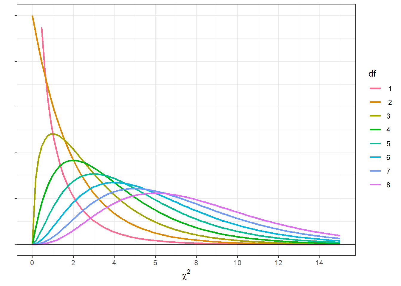
Notice how the shape of the distributions spread out and change shape with increasing degrees of freedom. This is because as we increase df, and therefore the number of squared z-scores, the sum will on average increase too.
Since the \(\chi^2\) distribution is known we can calculate the probability of obtaining our observed value of \(\chi^2\) if null hypothesis is true. For a \(\chi^2\) test for frequencies, The degrees of freedom is the number of categories minus one. For this example, df = 2- 1 = 1.
13.3 R’s pchisq function
Consistent with pnorm, pt and pF, R’s pchisq function finds the area below a given value. So to find the area above \(\chi^2\) = 4.9152 for df = 1 we subtract the result of pchisq from 1:
## [1] 0.0266213813.4 R’s qchisq function
Like qnorm, qt and qF, R’s qchisq function finds the value of \(\chi2\) for which a given proportion of the area lies below. So for our example, if \(\alpha\) = 0.05, the critical value of \(\chi^2\) for making our decision is:
## [1] 3.841459We reject \(H_{0}\) for any observed \(\chi^2\) value greater than 3.84.
Here’s an illustration of the pdf for \(\chi^2\) for df = 1 with the top 5 percent shaded in red and our observed value of \(\chi^2\) = 4.9152 shown as a vertical line.
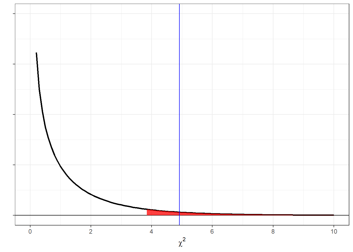
You can see that our observed value of \(\chi^2\) (4.9152) falls above the critical value of \(\chi^2\) (3.8415). Also, our p-value (0.0266) is less than \(\alpha\) = 0.05. We therefore reject \(H_{0}\) and conclude that the proportion of left and right handers in our class is significantly different than what is expected from the population.
13.5 Using chisq.test to run a \(\chi2\) test for frequencies
R has the chisq.test function that computes the values that we’ve done by hand. For our example we’ll load in the survey data and compute ‘fobs’ which is the frequency of the observed number of left and right handers in the class. This will be compared to prob = c(.1,.9) which is where we enter our population, or null hypothesis proportions.
survey <-read.csv("http://www.courses.washington.edu/psy315/datasets/Psych315W21survey.csv")
prob <- c(.1,.9)
fobs <- c(sum(survey$hand=="Left",na.rm = T),sum(survey$hand=="Right",na.rm = T))
chisq.out <- chisq.test(fobs,p=prob)
The important fields in the output of chisq.test are statistic which holds the observed \(\chi^2\) value, parameter which holds the degrees of freedom, expected which holds the computed expected frequencies, observed which holds the observed values (that we entered), and p.value.
13.6 APA format for the \(\chi^2\) test for independence
Here’s how to extract the fields in the output of chisq.test into generate a string in APA format:
sprintf('Chi-Squared(%d,N=%d) = %5.4f, p = %5.4f',
        chisq.out$parameter,
        sum(chisq.out$observed),
        chisq.out$statistic,
        chisq.out$p.value)
## [1] "Chi-Squared(1,N=152) = 4.9152, p = 0.0266"13.7 One or two tailed?
A common question for \(\chi^2\) tests is whether the test is one- or two-tailed. The \(\chi^2\) statistic is always nonnegative (because it is built from squared deviations), so the p-value is computed from the upper tail of the \(\chi^2\) distribution: large \(\chi^2\) values indicate a poor match between observed and expected frequencies.
At the same time, the test is non-directional: the observed frequency in a category can be too high or too low relative to the expected frequency, and either kind of discrepancy increases \(\chi^2\). So while the rejection region lives in the upper tail of the \(\chi^2\) distribution, the null hypothesis is violated by deviations in either direction.
13.8 Relationship between \(\chi^2\) test and the normal approximation to the binomial
You might have noticed that we already know a way of calculating the probability of obtaining 15.2 or more left-handers out of 152 students, assuming that 10 percent of the population is left-handed. That’s right - the normal approximation to the binomial.
Let’s compare:
Using the normal approximation with N = 152 and P = 0.1 , the number of left-handers will be distributed normally with a mean of
\[\mu = NP = (152 )(0.1 ) = 15.2\]
and a standard deviation of
\[\sigma = \sqrt{NP(1-P)} = \sqrt{(152 )(0.1 )(0.9 )} = 3.6986 \].
The Chi-squared test is a two-tailed test, so to conduct a two tailed test with the normal approximation to the binomial we need to find the probability of obtaining an observed value more extreme than 7 compared to 15.2 .
If we ignore the business of correcting for continuity, we can use pnorm to find this probability. First, we convert our observed frequency of left-handers to a z-score:
Then we convert our z-score to a p-value like we did back in the chapter on the normal distribution:
## [1] 0.02661626This number is very close to the p-value we got from the \(\chi^2\) test: 0.0266. In fact, the difference is only due to rounding error. Thus the \(\chi^2\) test with \(df = 1\) is mathematically equivalent to the normal approximation to the binomial. This means that the tests are the same if you don’t correct for continuity, which is that process of including the whole interval by subtracting and adding 0.5.
The \(\chi^2\) test is therefore actually not quite right. Also, remember that the normal approximation to the binomial is really best for larger sample sizes, like for n>20. But we typically run \(\chi^2\) tests for smaller values of n. values of n.
13.9 Comparing the \(\chi^2\) test to the binomial test
For two groups like this example, we can use the binomial distribution, which we can get from binom.test:
## [1] 0.02140999It’s close, but not exact. In most cases, the \(\chi^2\) test is a good enough approximation to the ‘exact’ solution. You really only run into trouble when your expected frequencies drop too low, say below 5 or so.
13.10 Example 2: Birthdays by month
Let’s see if the birthdays in this class are evenly distributed across months, or if there are some months for which students have significantly= more birthdays than others. For simplicity, we’ll assume that all months have equal probability, even though they vary in length. We’ll run a \(\chi^2\) test using an alpha value of 0.05.
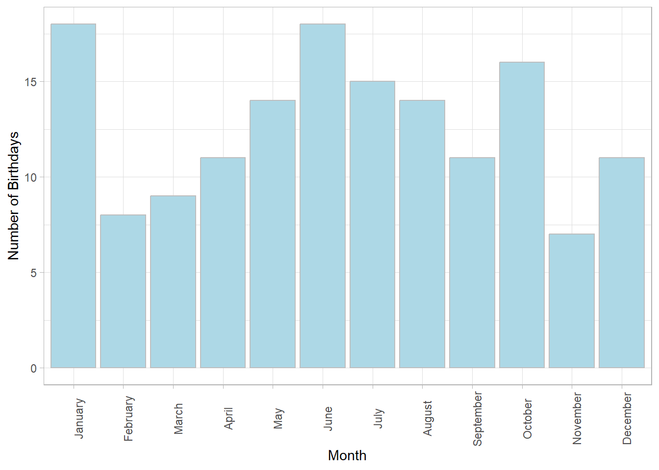
Here’s a table showing the number of birthdays for each month for all 152 students:
It looks kind of uneven. There are 18 students with birthdays in January and June but only 7 students with birthdays in November. A natural way to visualize this distribution is with a bar graph showing the frequency distribution:

To see if this distribution is significantly uneven we calculate the expected frequencies under the null hypothesis. Here we expect equal frequencies of \(\frac{152}{} = 12.6667\) birthdays per month . Note equal frequencies assumes that each month has an equal number of days. This assumption is close enough for this example, but how would you correct the expected frequencies to account for this?
Using our \(\chi^2\) formula:
\[\chi^{2} = \sum{\frac{(f_{obs}-f_{exp})^{2}}{f_{exp}}} = \frac{(18-12.6667)^{2}}{12.6667} ... + ... \frac{(11-12.6667)^{2}}{12.6667} = 12.0526\]
With months, the degrees of freedom is 11. Using pchisq we can find the p-value for our test:
## [1] 0.3597025Or, we can find the critical value of \(\chi^2\) using qnorm:
## [1] 19.67514We reject \(H_{0}\) for any observed \(\chi^2\) value greater than 19.68.
Here’s an illustration of the pdf for \(\chi^2\) for df = 11 with the top 5 percent shaded in red and our oberved value of \(\chi^2\) = 12.0526 shown as a vertical line.
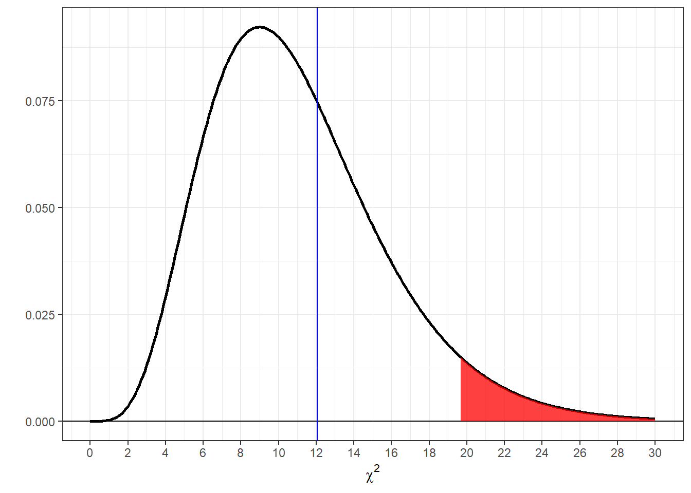
You can see that our observed value of \(\chi^2\) (12.0526) falls below the critical value of \(\chi^2\) (19.6751). Also, our p-value (0.3597) is greater than \(\alpha\) = 0.05. We therefore fail to reject \(H_{0}\) and conclude that the distribution of birthdays across months is not significantly different than what is expected from chance.
13.11 Conducting the same test with chisq.test
With the survey data loaded in from the previous example, running the \(\chi^2\) test for frequencies on the birth month data is pretty straightforward. The only new thing is the use of the function table to get a table of frequencies for birthdays across months, like we did in the chapter on descriptive statistics:
##
##   January  February     March     April       May      June      July    August
##        18         8         9        11        14        18        15        14
## September   October  November  December
##        11        16         7        11
We can then send this table into chisq.test. We could send in a list of expected probabilities, but by default, chisq.test assumes equal probabilities across categories:
##
##  Chi-squared test for given probabilities
##
## data:  dat
## X-squared = 12.053, df = 11, p-value = 0.3597
We can coerce the output of chisq.test into APA format just like we did for the first example:
sprintf('Chi-Squared(%d,N=%d) = %5.4f, p = %5.4f',
        chisq.out$parameter,
        sum(chisq.out$observed),
        chisq.out$statistic,
        chisq.out$p.value)
## [1] "Chi-Squared(11,N=152) = 12.0526, p = 0.3597"13.12 Effect size
There are a couple of definitions for effect size for the \(\chi^2\) chi-squared test for frequencies. The one that is used most commonly to calculate power is is called \(\psi\), or ‘psi’:
\[\psi = \sqrt{\frac{\chi^2}{N}}\]
Where \(N\) is the total sample size. From our first example (handedness):
\[\psi = \sqrt{\frac{\chi^{2}}{N}} = \sqrt{\frac{4.9152}{152}} = 0.1798\]
From our second example (birth months):
\[\psi = \sqrt{\frac{\chi^{2}}{N}} = \sqrt{\frac{12.0526}{152}} = 0.2816\]
\(\psi\) has the desirable quality that it is not influenced by sample size, so it can be used to compare effect sizes across experiments. However, since \(\chi^2\) increases with the number of categories (and df), so does \(\psi\), so we can’t use \(\psi\) on it’s own to determine if an effect is ‘small’, ‘medium’, or ‘large’.
An alternative measure of effect size is ‘Cramer’s V’, which puts the degrees of freedom in the denominator to offset the increase in df with \(\psi\):
\[V = \sqrt{\frac{\chi^2}{N \times df}}\]
If you look at the formulas you can see that there is a relation between \(\psi\) and \(V\):
\[V = \frac{\psi}{\sqrt{df}}\]
For V, 0.1 is considered small, 0.3 medium, and 0.5 is a large effect size.
From our first example (handedness):
\[V =\sqrt{\frac{\chi^{2}}{N \times df}} = \sqrt{\frac{4.9152}{(152)(1)}} = 0.1798\]
Which would be considered to be a small effect size.
From our second example (birth months):
\[V =\sqrt{\frac{\chi^{2}}{N \times df}} = \sqrt{\frac{12.0526}{(152)(11)}} = 0.0849\]
Which would also be considered to be a small effect size.
13.13 Power for the \(\chi^2\) test for frequencies
Power can be calculated with R using ‘pwr.chisq.test’. It requires the effect size \(\psi\) (called ‘w’ for some reason), the total sample size \(N\), the degrees of freedom, and the alpha value.
pwr.chisq.test works much like pwr.t.test for the t-test. To find the power for the first test on handedness:
The observed power for the first test can be found:
## [1] 0.6013325If you want to find the sample size that gives you a desired power of 0.8, pass in NULL for the sample size (N), and set power = .8:
The sample size needed is:
## [1] 242.788Power for the second example, on birth months is:
## [1] 0.6220806The sample sized needed to get a power of 0.8 is:
## [1] 211.8792