Chapter 10 Two Sample Independent Measures t-test
This t-test compares two means that are drawn from separate, or independent samples.
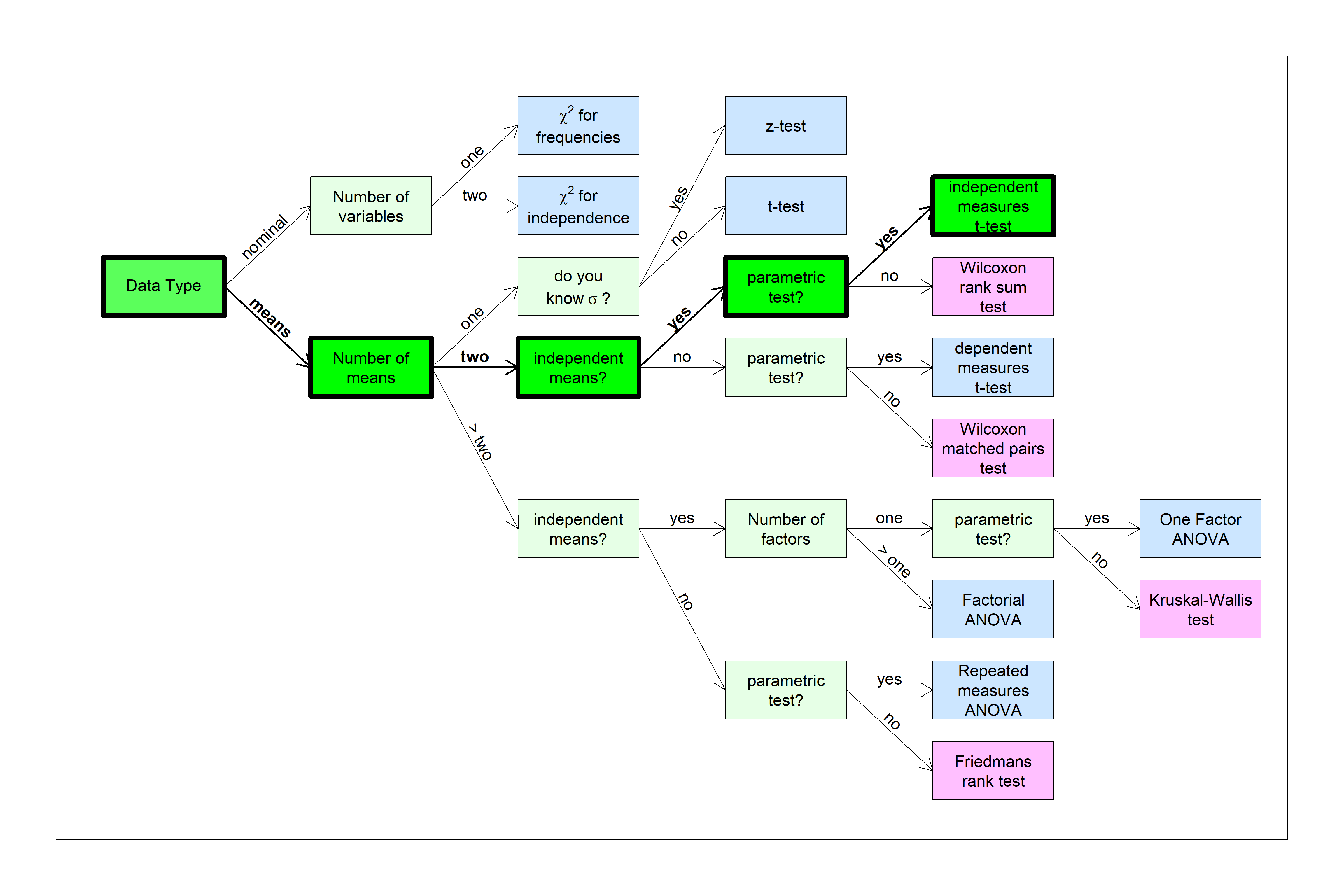
You can find this test in the flow chart here:
The null hypothesis is that the two means are drawn from populations with the same mean (or means that differ by some fixed amount). Formally we write the null hypothesis as:
\[H_{0}: (\mu_{x}-\mu_{y}) - \mu_{hyp} = 0\] Where \(x\) and \(y\) are the two populations that our samples are drawn from. Formally, the two-sample t-test estimates the probability of obtaining a difference between the observed means (or some expected difference \(\mu_{hyp}\)) if the null hypothesis is true. If this probability is small (less than \(\alpha\)), then we reject the null hypothesis in support of the alternative hypothesis that the population means for the two samples are not the same (or differ by more than \(\mu_{hyp}\)).
For the standard two-sample independent measures t-test, both the null and alternative hypotheses assume that the two population standard deviations are the same (even if we don’t know what that standard deviation is). If we drop this assumption of ‘equal variance’ then we run a similar test called ‘Welch’s t-test’, discussed later.
To conduct the test, we convert the two means and standard deviations into a test statistic which is drawn from a t-distribution under the null hypothesis:
\[t = \frac{\bar{x}-\bar{y} - \mu_{hyp}}{s_{\bar{x}-\bar{y}}}\]
Usually \(\mu_{hyp}\) is zero, which is when we are simply testing if the two means are significantly different from each other. So the simple case when we are comparing means to each other the calculation for t simplifies to the more familiar:
\[t = \frac{\bar{x}-\bar{y}}{s_{\bar{x}-\bar{y}}}\]
The denominator is called \(s_{\bar{x}-\bar{y}}\) because it represents the standard deviation of the difference between means, also called the pooled standard error of the mean. It is calculated by first combining the two sample standard deviations, \(s_x\) and \(s_y\) into a single number called the pooled standard deviation:
\[s_{p} = \sqrt{\frac{(n_{x}-1)s_{x}^{2}+(n_{y}-1)s_{y}^{2}}{(n_{x}-1)+(n_{y}-1)}}\]
\(s_{p}\) is a sort of complicated average of the two standard deviations. Technically, the calculation inside the square root is an average of the sample variances, weighted by their degrees of freedom. Importantly, \(s_{p}\) will always fall somewhere between the two sample standard deviations.
The denominator of the t-test, called the pooled standard error, is calculated from \(s_{p}\) by:
\[s_{\bar{x}-\bar{y}} = s_{p}\sqrt{\frac{1}{n_{x}} + \frac{1}{n_{y}}}\]
Where \(n_x\) and \(n_y\) are the two sample sizes. This is sort of like how we calculated the standard error from the sample standard deviation for the single sample t-test: \(s_{\bar{x}} = \frac{s_{x}}{\sqrt{n}}\).
You can go straight to the pooled standard error of the mean in one step if you prefer:
\[s_{\bar{x}-\bar{y}} = \sqrt{\frac{(n_{x}-1)s_{x}^{2}+(n_{y}-1)s_{y}^{2}}{(n_{x}-1)+(n_{y}-1)}(\frac{1}{n_{x}} + \frac{1}{n_{y}})}\]
Note: if the two sample sizes are the same (\(n_{x} = n_{y} = n\)), then the pooled standard error of the mean simplifies to:
\[s_{\bar{x}-\bar{y}} = \sqrt{\frac{s_{x}^{2}+s_{y}^{2}}{n}}\]
The degrees of freedom of the independent means t-test is the sum of the degrees of freedom for each mean:
\[df = (n_{x}-1)+(n_{y}-1) = n_{x}+n_{y}-2\]
10.1 Example 1: one-tailed test for independent means, equal sample sizes
Suppose you’re a 315 Stats professor who has recently introduced a new textbook. You want to know if this new textbook are helping students learn. You do this by comparing Exam 2 scores from course taught this year with tutorials to the course taught last year without the textbook.
In this year, the 81 Exam 2 scores had a mean of 76.9345 and a standard deviation of 26.9491. The 81 Exam 2 scores in last year had a mean of 67.4122 and a standard deviation of 27.5612792. Let’s run a hypothesis test to determine of the mean Exam 2 scores from this year is significantly greater than from last year. Use \(\alpha\) = 0.05.
First we calculate the pooled standard error of the mean. Since the sample sizes are the same (\(n_{x} = n_{y}\) = 81):
\[s_{\bar{x}-\bar{y}} = \sqrt{\frac{s_{x}^{2}+s_{y}^{2}}{n}} = \sqrt{\frac{26.9491^{2}+27.5613^{2}}{81}} = 4.283\]
Our t-statistic is therefore:
\[t = \frac{\bar{x} - \bar{y}}{s_{\bar{x}-\bar{y}}}=\frac{76.9345 - 67.4122}{4.2830} = 2.2233\]
This is a one-tailed t-test with df = \(81+81-2 = 160\) and \(\alpha\) = 0.05. We can find our p-value using R’s pt function:
## [1] "1-pt(2.2233,160)"## [1] 0.0137983Our p-value is less than \(\alpha = 0.05\). We therefore reject \(H_{0}\) and conclude that the mean Exam 2 scores from this year is significantly greater than from last year.
To state our conclusions using APA format, we’d state:
“The exam scores from this year for the Exam 2 scores (M = 76.9, SD = 26.9) are significantly greater than the exam scores from last year (M = 67.4, SD = 27.6), t(160) = 2.2, \(p = 0.0138\).”
10.2 Error Bars
For tests of independent means it’s useful to plot our means as bars on a bar graph with error bars representing \(\pm\) one standard error of the mean. We calculate the standard error of the mean for each sample the usual way by dividing each sample standard deviation by the square root of its sample size:
For this year,
\[s_{\bar{x}} = \frac{s_{x}}{\sqrt{n}} = \frac{26.9491}{\sqrt{81}} = 2.9943\]
and for last year,
\[s_{\bar{y}} = \frac{s_{y}}{\sqrt{n}} = \frac{27.5613}{\sqrt{81}} = 3.0624\]
The error bars are drawn by moving up and down one standard error of the mean (\(s_{\bar{x}}\)) for each mean (\(\bar{x}\)):
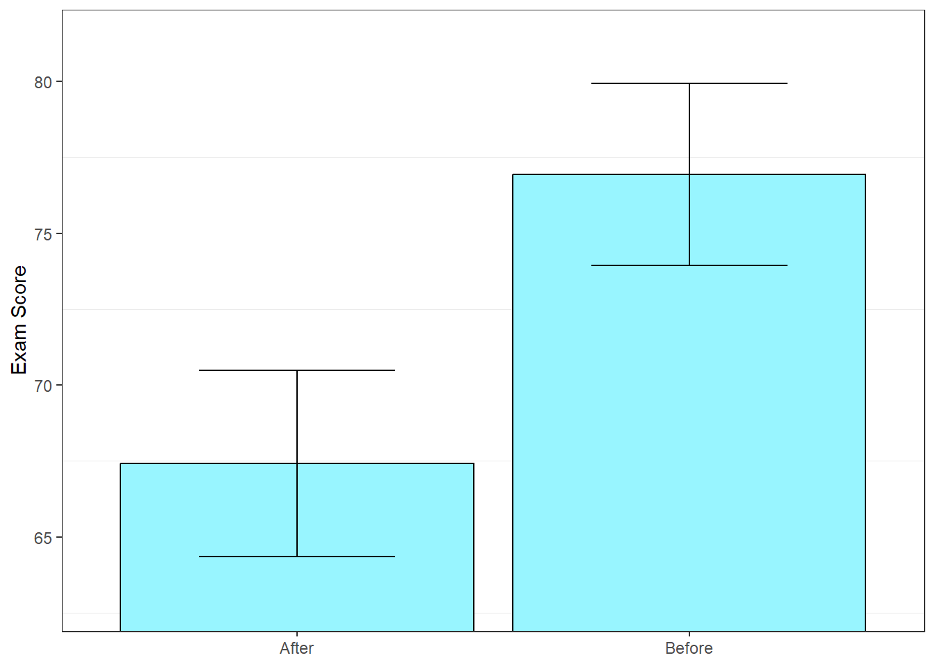
Bar graphs with error bars are useful for visualizing the significance of the difference between means.
Remember this rule of thumb: If the error bars overlap, then a one-tailed t-test will fail to reject \(H_{0}\) with \(\alpha\) = .05. A one-tailed test with \(\alpha\) = .05 is the most liberal test, so any other test will also need a gap to reach significance. You’ll need a larger gap between the error bars to reach significance for a two-tailed test, and/or for smaller values of \(\alpha\), like .01.
10.3 Example 2: Heights of women with tall and less tall mothers
Suppose you want to test the hypothesis that women with tall mothers are different than women with less tall mothers. We’ll use our Psych 315 data and divide the students into women with mothers that are taller and shorter than the median of of 64 inches (5 feet 4 inches). The height of the 55 women with tall mothers has a mean of 65.9273 inches and a standard deviation of 2.5953 inches. The height of the 63 women with less tall mothers has a mean of 63.6349 inches and a standard deviation of 2.5546 inches. Are these heights significantly different? Use alpha = 0.01.
Since our sample sizes are different, we have to use the more complicated formula for the pooled standard error of the mean:
\(s_{p} = \sqrt{\frac{(n_{x}-1)s_{x}^{2}+(n_{y}-1)s_{y}^{2}}{(n_{x}-1)+(n_{y}-1)}} = \sqrt{\frac{(55-1)(2.5953)^{2}+(63-1)(2.5546)^{2}}{(55-1)+(63-1)}} = 2.5736\)
\(s_{\bar{x}-\bar{y}} = s_{p}\sqrt{\frac{1}{n_{x}} + \frac{1}{n_{y}}} = 2.5736\sqrt{\frac{1}{55} + \frac{1}{63}} = 0.4749\)
Our t-statistic is
\(t = \frac{\bar{x} - \bar{y}}{s_{\bar{x}-\bar{y}}}=\frac{65.9273 - 63.6349}{0.4749} = 4.8267\)
Using R’s pt function, the p-value for this two-tailed test is:
## [1] "2*(1-pt(abs(4.8267),116))"## [1] 4.268748e-06Our p-value is less is than \(\alpha\) = 0.01. We therefore reject \(H_{0}\) and conclude that the mean height height of the women with tall mothers height is statistically different from the heights of height of the women with less tall mothers height.
10.4 Using R’s t.test from the data
This was all done by hand with the given means and standard deviations. Now we’ll use R to load in the data set and conduct the test using R’s t.test function. First we load in the survey data and pull out the heights of the mothers of the students that identify as women, which are in the field ‘mheight’
survey <- read.csv("http://www.courses.washington.edu/psy315/datasets/Psych315W21survey.csv")
mheight <- survey$mheight[!is.na(survey$mheight) & survey$gender=="Woman" ]
Next, we’ll find the median of the mother’s height and divide the women’s heights into two groups, the variable x will hold the heights of the women with mother’s heights are greater than the median, and y will hold the heights of the women less than or equal to the median:
# Find the heights of the women students who's mother's aren't NA's:
height <- survey$height[!is.na(survey$mheight) & survey$gender=="Woman"]

# Find the heights of students that identify as women who's mothers are taller than the median.  Call them 'x'
x <- na.omit(height[mheight>median(mheight)])

# Find the heights of students that identify as women who's mother's heights are less than or equal to the median.  Call them 'y'
y <- na.omit(height[mheight<=median(mheight)])
Now we’re ready for t.test. If you send in both x and y, t.test assumes that we’re running a two-sample independent measures t-test. The var.equal = TRUE tells R to use the pooled standard deviation formula. If var.equal = FALSE, t.test runs the Welch Two Sample t-test I’ll describe later.
Here’s where you can find the information needed to report your results in APA format:
## [1] "t(116) = 4.83, p = 0.0000043"10.4.1 Alternate way to run t.test: formula and ‘long format’
We ran the t.test function by inputting the two vectors, x and y as the fist two arguments. But often your data is not organized as two vectors like this. For example, if you’re reading these two vectors from a csv file, the data will most likely be organized in ‘long’ format, where each student has a row, and a second column determines which category the student belongs to (e.g. ‘tall mothers’). You can find the same data from the t-test above in a csv file organized in long format. Here’s how to load it in:
heights.long <- read.csv("http://www.courses.washington.edu/psy524a/datasets/HeightsLongFormat.csv")Here’s what the data structure looks like:
| mother | height |
|---|---|
| tall | 65 |
| tall | 67 |
| tall | 69 |
| tall | 71 |
| tall | 66 |
| tall | 62 |
| tall | 67 |
| tall | 68 |
| tall | 67 |
| tall | 68 |
| tall | 66 |
| tall | 67 |
| tall | 63 |
| tall | 62 |
| tall | 61 |
| tall | 69 |
| tall | 68 |
| tall | 69 |
| tall | 68 |
| tall | 70 |
| tall | 62 |
| tall | 64 |
| tall | 62 |
| tall | 67 |
| tall | 68 |
| tall | 68 |
| tall | 62 |
| tall | 62 |
| tall | 68 |
| tall | 64 |
| tall | 67 |
| tall | 66 |
| tall | 66 |
| tall | 65 |
| tall | 66 |
| tall | 67 |
| tall | 64 |
| tall | 62 |
| tall | 67 |
| tall | 62 |
| tall | 68 |
| tall | 64 |
| tall | 65 |
| tall | 71 |
| tall | 68 |
| tall | 68 |
| tall | 63 |
| tall | 64 |
| tall | 63 |
| tall | 66 |
| tall | 65 |
| tall | 66 |
| tall | 69 |
| tall | 69 |
| tall | 65 |
| not tall | 64 |
| not tall | 63 |
| not tall | 60 |
| not tall | 66 |
| not tall | 62 |
| not tall | 66 |
| not tall | 61 |
| not tall | 62 |
| not tall | 61 |
| not tall | 64 |
| not tall | 62 |
| not tall | 65 |
| not tall | 60 |
| not tall | 62 |
| not tall | 65 |
| not tall | 62 |
| not tall | 61 |
| not tall | 65 |
| not tall | 64 |
| not tall | 61 |
| not tall | 66 |
| not tall | 64 |
| not tall | 63 |
| not tall | 62 |
| not tall | 61 |
| not tall | 65 |
| not tall | 62 |
| not tall | 63 |
| not tall | 63 |
| not tall | 63 |
| not tall | 72 |
| not tall | 68 |
| not tall | 61 |
| not tall | 62 |
| not tall | 59 |
| not tall | 63 |
| not tall | 62 |
| not tall | 65 |
| not tall | 70 |
| not tall | 63 |
| not tall | 66 |
| not tall | 60 |
| not tall | 65 |
| not tall | 65 |
| not tall | 65 |
| not tall | 66 |
| not tall | 67 |
| not tall | 63 |
| not tall | 65 |
| not tall | 60 |
| not tall | 64 |
| not tall | 61 |
| not tall | 68 |
| not tall | 64 |
| not tall | 64 |
| not tall | 67 |
| not tall | 65 |
| not tall | 63 |
| not tall | 61 |
| not tall | 68 |
| not tall | 65 |
| not tall | 63 |
| not tall | 61 |
The data has two colunns, one for what category the student is in (based on their mother’s height: ‘tall’ and ‘not tall’ ) and the second column is the student’s height. To run a t-test on data in long format we could pull out the numbers into two vectors, x and y. But an easier way is to define the test as a ‘formula’.
What we’re really doing with this t-test is trying to predict the student’s heights based on their mother’s heights, and measuring, with a p-value, the quality of this prediction. In R, we write this as height ~ mother, which reads as predicting the continuous variable ‘height’ from the categorical variable ‘mother’. Here’s how to run the t-test using this formula:
out <- t.test(height~mother ,data = heights.long,alternative = "two.sided",var.equal = TRUE,alpha = .01)
sprintf('t(%g) = %4.2f, p = %5.7f',out$parameter,out$statistic,out$p.value)
## [1] "t(116) = -4.83, p = 0.0000043"You can verify that we get the same results as sending the data as ‘x’ and ‘y’ vectors. Later on when we get into regression and ANOVA we’ll be using the formula method extensively.
10.5 Bar plots with Error Bars in R
To generate the bar plots, we’ll use R’s ggplot function from the ‘ggplot2’ package. The first step is to generate a ‘data frame’ that holds our statistics:
summary <- data.frame(
  mean = c(mean(x),mean(y)),
  n = c(length(x),length(y)),
  sd = c(sd(x),sd(y)),row.names = c('Tall','Less Tall'))
# use these to calculate the two standard errors of the mean
summary$sem <- summary$sd/sqrt(summary$n)
We’ve created a nice table of our summary statistics:
##               mean  n       sd       sem
## Tall      65.92727 55 2.595256 0.3499442
## Less Tall 63.63492 63 2.554576 0.3218463
This will define the y-axis limits for the bar graph. For most bar graphs with ratio scale measures we include zero, but bar graphs with error bars are an exception because we want to compare the differences between the means, not how far the means are from zero. The graph looks nice if we add about \(\frac{1}{2}\) of a standard error above and below the error bars:
We’re ready to call ggplot. ggplot is a very flexible function and takes a while to get used to. The first argument is the data frame that we created. The second defines what fields of the data frame correspond to the x and y-axis variables. geom_col tells ggplot that we’re drawing a bar graph. geom_errorbar adds error bars of the specified lengths. I find it most useful to take existing ggplot code and editing them, rather than starting from scratch. So you can use this as a starting point for all of your bar graphs with error bars.
# Plot bar graph with error bar as one standard error (standard error of the mean/SEM)
ggplot(summary, aes(x = row.names(summary), y = mean)) +
  geom_col(position = position_dodge(), fill="cadetblue1",color = "black") +
  geom_errorbar(aes(ymin=mean-sem, ymax=mean+sem),width = .5) +
  xlab("Mother's Height") +
  theme_bw() +
  theme(panel.grid.major = element_blank()) +
  scale_y_continuous(name = "Student's Height (in)") +
  coord_cartesian(ylim=ylimit)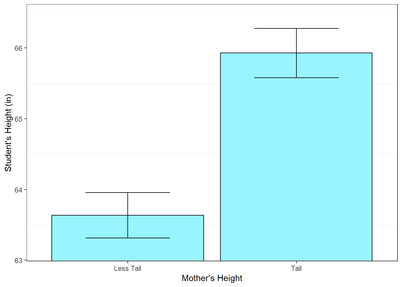
Notice the large gap between the error bars. Hence our small p-value.
10.6 Effect size
The effect size for an independent measures t-test is Cohen’s d again. This time it’s measured as:
\(d = \frac{|\bar{x}-\bar{y} - (\mu_{x}-\mu_{y})_{hyp}|}{s_{p}}\)
Or more commonly when \((\mu_{x}-\mu_{y})_{hyp}\) = 0:
\(d = \frac{|\bar{x}-\bar{y}|}{s_{p}}\)
where, from above, the denominator is the pooled standard deviation:
\(s_{p} = \sqrt{\frac{(n_{x}-1)s_{x}^{2}+(n_{y}-1)s_{y}^{2}}{(n_{x}-1)+(n_{y}-1)}}\)
and for equal sizes:
\(s_{p} = \sqrt{\frac{s_{x}^{2}+s_{y}^{2}}{2}}\)
For the first example on test scores:
\(d = \frac{|\bar{x} - \bar{y}|}{s_{p}}= \frac{|76.9345 - 67.4122|}{27.2569} = 0.3494\)
This is a small effect size.
For the second example on student’s heights:
\(d = \frac{|\bar{x} - \bar{y}|}{s_{p}}= \frac{|65.9273 - 63.6349|}{2.5736} = 0.8907\)
Which is considered to be a large effect size.
10.6.1 Calculating effect size using R’s cohen’s d
The package ‘rstatix’ provides some useful tools for calculating summary statistics, including cohen’s d. You’ll need to install the package using R’s install.packages function, and then add the line library(rstatix) in your code. Once done, you can calculate Cohen’s d from long-formatted data like this:
heights.long <- read.csv("http://www.courses.washington.edu/psy524a/datasets/HeightsLongFormat.csv")

cohen_out <- cohens_d(formula = height ~ mother,data = heights.long , var.equal = TRUE)
Note that the order of the arguments in t.test is ‘formula’ followed by ‘data’, but the order for Cohen’s d is ‘data’ followed by ‘formula’. This lack of standardization is a classic problem in open-source languages. So to be safe, you can always send in the arguments in your own order as long as you name them (e.g. formula = height~mother).
The field effsize holds Cohen’s d, though it can be negative depending on the order of the nominal-scale values which are ordered alphabetically. (‘not tall’ comes before ‘tall’ in this example). So take the absolute value just in case:
## Cohen's d: 0.890710.7 Power for the two-sample independent measures t-test
Power calculations for the independent mean t-test are conceptually the same as for the t-test for one mean. It’s still the probability of correctly rejecting \(H_{0}\). Power for a two-sample independent measures t-test is easy to calculate in R using power.t.test. We just have to specify type = 'two.sample'. The only weird thing is that the sample size - it takes in just one number, which is calculated by:
\[ n = \frac{2}{\frac{1}{n_x} + \frac{1}{n_y}} \] Which is the ‘harmonic mean’ of \(n_x\) and \(n_y\). If the sample sizes are equal, then it reduces to \(n = n_x = n_y\).
For our first example on exam scores, which was a one-sided test, the effect size was d = 0.3494, \(\alpha\) = 0.05, and the ‘sample size’ is:
\[ n = \sqrt{\frac{1}{n_x} + \frac{1}{n_y}} = \sqrt{\frac{1}{81} + \frac{1}{81}} = 81 \]
the observed power is found with:
power.out <- power.t.test(n=81,delta=0.3494,sig.level=0.05,type ='two.sample',alternative = 'one.sided')## [1] 0.7154228This means that with this observed effect size and sample size, there is about a 72% chance of rejecting \(H_{0}\) for any given experiment.
For the second example, on women’s heights, which was a two-sided test with an average sample size of `r, an effect size of d = 0.8907, \(\alpha\) = 0.01, and a combined sample size of:
\[ n = \sqrt{\frac{1}{n_x} + \frac{1}{n_y}} = \sqrt{\frac{1}{55} + \frac{1}{63}} = 58.73 \]
the observed power is found with:
power.out <- power.t.test(n=58.73,delta=0.8907,sig.level=0.01,type ='two.sample',alternative = 'two.sided')## [1] 0.9854064The set of power curves from the chapter on power include curves for independent means and can be found at:
10.8 Welch’s t-test for Unequal population variances
As described above, the pooled standard deviation, \(s_{p}\), assumes that the variances of the two populations that we’re drawing from are equal. But if the population variances are unequal, then the standard two-sample t-tests can lead to inflated type I errors.
If we want to drop this assumption we have to resort to an alternate version of the two-sample t-test most commonly called ‘Welch’s t-test’.
The logic is the same as the standard two-sample t-test, but there are two changes. First, the denominator of the t-test changes to:
\(s_{\bar{x}-\bar{y}} = \sqrt{\frac{s_x^{2}}{n_x} + \frac{s_y^{2}}{n_y}}\)
Which is actually simpler than for the regular t-test. The second change is to ‘adjust’ the degrees of freedom to:
\[df = \frac{\left(\frac{s_x^{2}}{n_x}+\frac{s_y^{2}}{n_y}\right)^{2}}{\frac{\left(\frac{s_x^{2}}{n_x}\right)^{2}}{n_{x}-1}+ \frac{\left(\frac{s_y^{2}}{n_y}\right)^{2}}{n_{y}-1}}\]
From our second example about womens’ heights:
\(df = \frac{\left(\frac{s_x^{2}}{n_x}+\frac{s_y^{2}}{n_y}\right)^{2}}{\frac{\left(\frac{s_x^{2}}{n_x}\right)^{2}}{n_{x}-1}+ \frac{\left(\frac{s_y^{2}}{n_y}\right)^{2}}{n_{y}-1}} = \frac{\left(\frac{2.5953^{2}}{55}+\frac{2.5546^{2}}{63}\right)^{2}}{\frac{\left(\frac{2.5953^{2}}{55}\right)^{2}}{55-1}+\frac{\left(\frac{2.5546^{2}}{63}\right)^{2}}{63-1}} = 113.3523\)
The degrees of freedom for the Welch test isn’t usually a whole number, which is weird. But R and other software can deal with calculating p-values for df’s that are not integers.
The new t-statistic is:
\(t = \frac{\bar{x} - \bar{y}}{s_{\bar{x}-\bar{y}}}=\frac{65.9273 - 63.6349}{0.4754} = 4.8215\)
The p-value for the Welch test is 0.00000446
Recall that treated with equal variance, the original df was 116, the original t-statistic was 4.8267 and the original p-value was 0.00000427. Not much of a change.
10.8.1 Effect size for the Welch Test
The denominator for Cohen’s d for the regular two-sample independent measures t-test is the pooled standard deviation. For the Welch test we skipped the pooling step and went straight to the denominator of the t-test, \(s_{x,y}\).
For the denominator of Welch’s test we pool the standard deviations by taking the square root of the mean of the variances:
\[ \sqrt{\frac{s_{x}^{2}+s_{y}^{2}}{2}}\] So for our example, Cohen’s d for the Welch test is:
\[d = \frac{|\bar{x} - \bar{y}|}{\sqrt{\frac{s_{x}^2+s_{y}^2}{2}}}=\frac{|65.9273 - 63.6349|}{\sqrt{\frac{2.5953^2+2.5546^2}{2}}} = 0.8902\]
This is really close to the value if we assume equal variance d = 0.8907.
10.8.1.1 Effect size for the Welch test using R’s ‘cohens_d’
All we need to do is change var.equal from TRUE to FALSE (or just leave it out, since ‘FALSE’ is the default.)
cohen_out <- cohens_d(formula = height ~ mother,data = heights.long , var.equal = FALSE)

cat(sprintf("Cohen's d: %0.4f",abs(cohen_out$effsize)))
## Cohen's d: 0.890210.8.2 When to use the Welch test?
Statisticians will tell you to use the Welch test when you can’t assume that the variances of the two populations are equal. But then they’ll tell you that you shouldn’t run a hypothesis test on the difference between the sample variances (called a ‘Levene’s’ test) to determine if you should run a Welch test. Instead, you should only choose the Welch test ahead of time when you somehow know that the variances of the populations might not be equal.
Interestingly, in simulations with unequal variances, the Welch test corrects for the inflated type-I errors, but there is no loss in the power when there is a true difference between the population means.
This seems like something-for-nothing, so real question is when should we not use the Welch test? Well, current opinion seems to be moving toward dropping the regular two-sample t-test and always using the Welch test. In future years I’ll probably drop the standard t-test and teach with the Welch test entirely. But for now when I ask you to conduct an independent measures t-test we’ll use the standard t-test method.
For an interesting discussion on when to (or always) use the Welch test see:
http://daniellakens.blogspot.com/2015/01/always-use-welchs-t-test-instead-of.html
You can test out the effect of unequal variances yourself by playing around with the parameters in the R-script: