Chapter 6 Hypothesis Testing: the z-test
We’ve all had the experience of standing at a crosswalk waiting staring at a pedestrian traffic light showing the little red man. You’re waiting for the little green man so you can cross. After a little while you’re still waiting and there aren’t any cars around. You might think ‘this light is really taking a long time’, but you continue waiting. Minutes pass and there’s still no little green man. At some point you come to the conclusion that the light is broken and you’ll never see that little green man. You cross on the little red man when it’s clear.
You may not have known this but you just conducted a hypothesis test. When you arrived at the crosswalk, you assumed that the light was functioning properly, although you will always entertain the possibility that it’s broken. In terms of hypothesis testing, your ‘null hypothesis’ is that the light is working and your ‘alternative hypothesis’ is that it’s broken. As time passes, it seems less and less likely that light is working properly. Eventually, the probability of waiting this long assuming the light is functioning properly becomes so low that you reject the null hypothesis.
This sort of reasoning is the backbone of hypothesis testing and inferential statistics. It’s also the point in the course where we turn the corner from descriptive statistics to inferential statistics. Rather than describing our data in terms of means and plots, we will now start using our data to make inferences, or generalizations, about the population that our samples are drawn from. In this course we’ll focus on standard hypothesis testing where we set up a null hypothesis and determine the probability of our observed data under the assumption that the null hypothesis is true (the much maligned p-value). If this probability is small enough, then we conclude that our data suggests that the null hypothesis is false, so we reject it.
In this chapter, we’ll introduce hypothesis testing with examples from a ‘z-test’, when we’re comparing a single mean to what we’d expect from a population with known mean and standard deviation. In this case, we can convert our observed mean into a z-score for the standard normal distribution. Hence the name z-test.
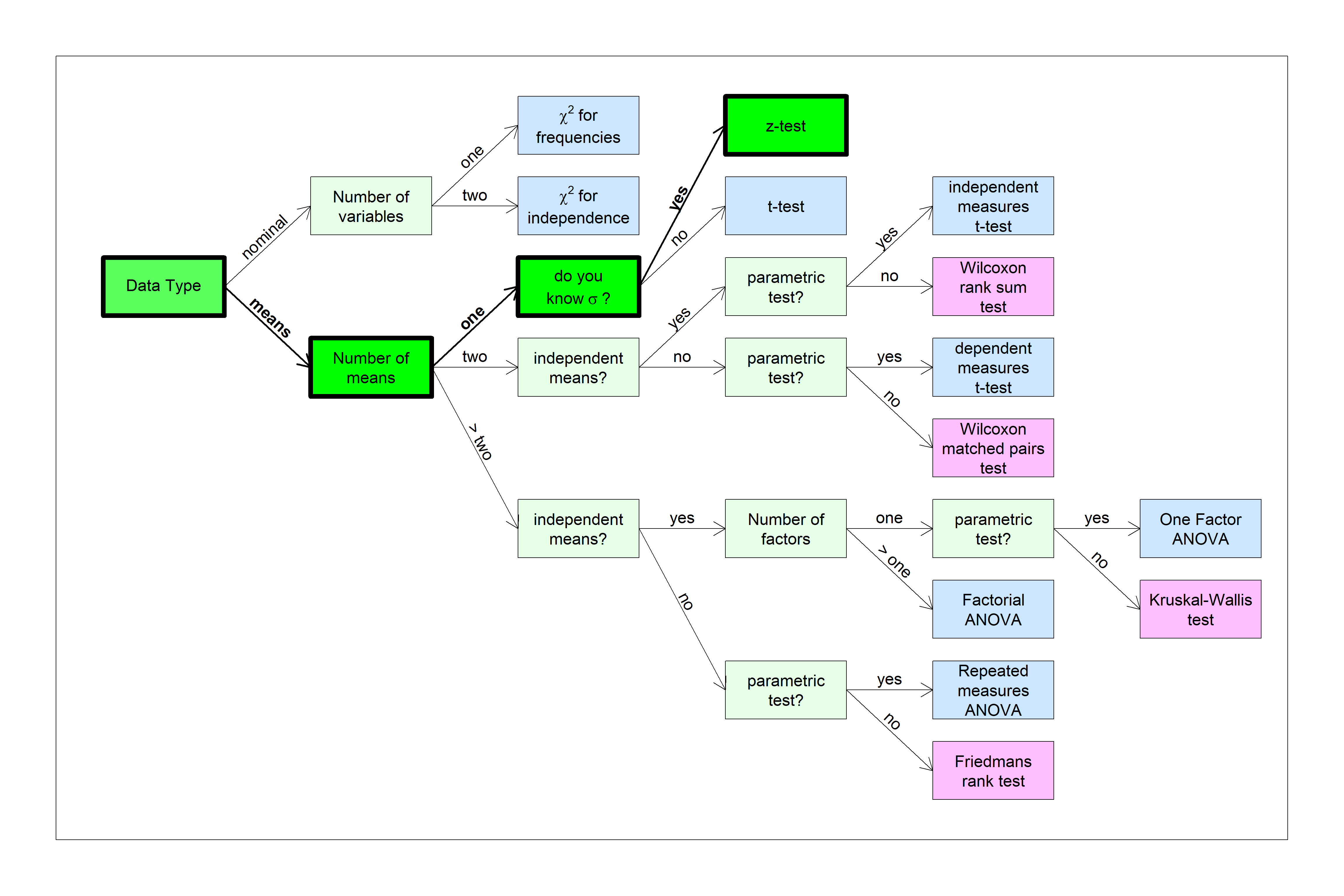
It’s time to introduce the hypothesis test flow chart. It’s pretty self explanatory, even if you’re not familiar with all of these hypothesis tests. The z-test is (1) based on means, (2) with only one mean, and (3) where we know \(\sigma\), the standard deviation of the population. Here’s how to find the z-test in the flow chart:
6.1 Women’s height example
Let’s work with the example from the end of the last chapter where we started with the fact that the heights of US women has a mean of 63 and a standard deviation of 2.5 inches. We calculated that the average height of the 122 women in Psych 315 is 64.7 inches. We then used the central limit theorem and calculated the probability of a random sample 122 heights from this population having a mean of 64.7 or greater is 2.4868996^{-14}. This is a very, very small number.
Here’s how we do it using R:
mu <- 63  # population mean
sigma <- 2.5 # population standard deviation
alpha <- .05

survey <- read.csv("http://www.courses.washington.edu/psy315/datasets/Psych315W21survey.csv")

women.height <- na.omit(survey$height[survey$gender=="Woman"])
x <- mean(women.height)   # sample mean
n <-length(women.height)  # sample size
sem <- sigma/sqrt(n)      # standard error of the mean

p <- 1-pnorm(x,mu,sem)    # p-value from normal distribution
print(sprintf('p = %1.15f',p))
## [1] "p = 0.000000000000025"Let’s think of our sample as a random sample of UW psychology students, which is a reasonable assumption since all psychology students have to take a statistics class. What does this sample say about the psychology students that are women at UW compared to the US population? It could be that these psychology students at UW have the same mean and standard deviation as the US population, but our sample just happens to have an unusual number of tall women, but we calculated that the probability of this happening is really low. Instead, it makes more sense that the population that we’re drawing from has a mean that’s greater than the US population mean. Notice that we’re making a conclusion about the whole population of women psychology students based on our one sample.
Using the terminology of hypothesis testing, we first assumed the null hypothesis that UW women psych students have the same mean as the US population. The null hypothesis is written as:
\[ H_{0}: \mu = 63 \] In this example, our alternative hypothesis is that the mean of our population is larger than the mean of null hypothesis population. We write this as:
\[ H_{A}: \mu > 63 \]
Next, after obtaining a random sample and calculate the mean, we calculate the probability of drawing a mean this large (or larger) from the null hypothesis distribution.
If this probability is low enough, we reject the null hypothesis in favor of the alternative hypothesis. When our probability allows us to reject the null hypothesis, we say that our observed results are ‘statistically significant’.
In statistics terms, we never say we ‘accept that alternative hypothesis’ as true. All we can say is that we don’t think the null hypothesis is true. I know it’s subtle, but in science can never prove that a hypothesis is true or not. There’s always the possibility that we just happened to grab an unusual sample from the null hypothesis distribution.
6.2 The hated p<.05
The probability that we obtain our observed mean or greater given that the null hypothesis is true is called the p-value. How improbable is improbable enough to reject the null hypothesis? The p-value for our example above on women’s heights is astronomically low, so it’s clear that we should reject \(H_{0}\).
The p-value that’s on the border of rejection is called the alpha (\(\alpha\)) value. We reject \(H_{0}\) when our p-value is less than \(\alpha\).
You probably know that the most common value of alpha is \(\alpha = .05\).
The first publication of this value dates back to Sir Ronald Fisher, in his seminal 1925 book Statistical Methods for Research Workers where he states:
“It is convenient to take this point as a limit in judging whether a deviation is considered significant or not. Deviations exceeding twice the standard deviation are thus formally regarded as significant.” (p. 47)
If you read the chapter on the normal distribution, then you should know that 95% of the area under the normal distribution lies within \(\pm\) two standard deviations of the mean. So the probability of obtaining a sample that exceeds two standard deviations from the mean (in either direction) is .05.
6.3 IQ example
Let’s do an example using IQ scores. IQ scores are normalized to have a mean of 100 and a standard deviation of 15 points. Because they’re normalized, they are a rare example of a population which has a known mean and standard deviation. In the next chapter we’ll discuss the t-test, which is used in the more common situation when we don’t know the population standard deviation.
Suppose you have the suspicion that graduate students have higher IQ’s than the general population. You have enough time to go and measure the IQ’s of 25 randomly sampled grad students and obtain a mean of 105. Is this difference between our this observed mean and 100 statistically significant using an alpha value of \(\alpha = 0.05\)?
Here the null hypothesis is:
\[ H_{0}: \mu = 100\]
And the alternative hypothesis is:
\[ H_{A}: \mu > 100 \]
We know that the parameters for the null hypothesis are:
\[ \mu = 100 \] and \[ \sigma = 15 \]
From this, we can calculate the probability of observing our mean of 105 or higher using the central limit theorem and what we know about the normal distribution. Specifically, under the null hypothesis, the sampling distribution of the mean is normal with a mean of \(\mu\) and a standard deviation of \(\sigma_{\bar{x}} = \frac{\sigma_{x}}{\sqrt{n}}\)
\[ \sigma_{\bar{x}} = \frac{\sigma_{x}}{\sqrt{n}} = \frac{15}{\sqrt{25}} = 3 \] From this, we can calculate the probability of our observed mean using R’s ‘pnorm’ function. Here’s how to do the whole thing in R.
mu <- 100 # null hypothesis population mean
sigma <- 15 # null hypothesis population standard deviation
n <- 25  # sample size
x_bar <- 105  # sample mean

sem <- sigma/sqrt(n)  # standard error or the mean

p_value <- round(1-pnorm(x_bar,mu,sem),4)
print(sprintf('p = %5.4f',p_value))
## [1] "p = 0.0478"Since our p-value of 0.0478 is (just barely) less than our chosen value of \(\alpha = 0.05\) as our criterion, we reject \(H_{0}\) for this (contrived) example and conclude that our observed mean of 105 is significantly greater than 100, so our study suggests that the average graduate student has a higher IQ than the overall population.
You should feel uncomfortable making such a hard, binary decision for such a borderline case. After all, if we had chosen our second favorite value of alpha, \(\alpha = .01\), we would have failed to reject \(H_{0}\). This discomfort is a primary reason why statisticians are moving away from this discrete decision making process. Later on we’ll discuss where things are going, including reporting effect sizes, and using confidence intervals.
6.4 Alpha values vs. critical values
Using R’s qnorm function, we can find the z-score for which only 5% of the area lies above:
## [1] 1.644854So the probability of a randomly sampled z-score exceeding 1.644854 is less than 5%. It follows that if we convert our observed mean into z-score values, we will reject \(H_{0}\) if and only if our z-score is greater than 1.644854. This value is called the ‘critical value’ because it lies on the boundary between rejecting and failing to reject \(H_{0}\).
In our last example, the z-score for our observed mean is:
\[ z = \frac{X-\mu}{\frac{\sigma}{\sqrt{n}}} = \frac{105 - 100}{3} = 1.67 \] Our z-score is just barely greater than the critical value of 1.644854, which makes sense because our p-value is just barely less than 0.05.
Sometimes you’ll see textbooks will compare critical values to observed scores for the decision making process in hypothesis testing. This dates back to days were computers were less available and we had to rely on tables instead. There wasn’t enough space in a book to hold complete tables which prohibited the ability to look up a p-value for any observed value. Instead only critical values for specific values of alpha were included. If you look at really old papers, you’ll see statistics reported as \(p<.05\) or \(p<.01\) instead of actual p-values for this reason.
It may help to visualize the relationship between p-values, alpha values and critical values like this:
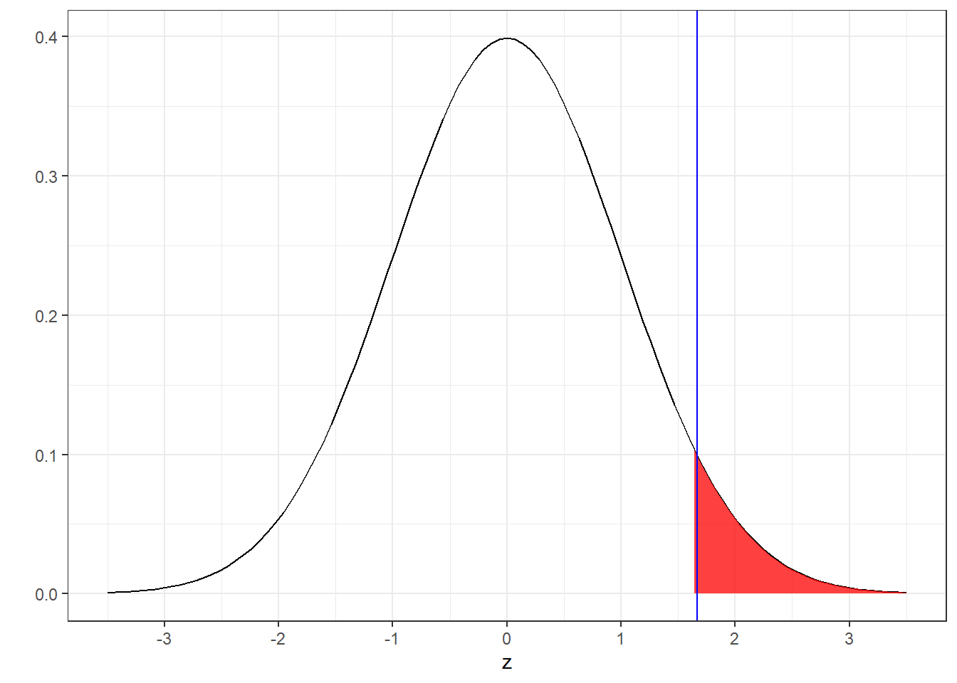
The red shaded region is the upper 5% of the standard normal distribution which starts at the critical value of z=1.644854. This is sometimes called the ‘rejection region’. The blue vertical line is drawn at our observed value of z=1.67. You can see that the red line falls just inside the rejection region, so we Reject \(H_{0}\)!
6.5 One vs. two-tailed tests
Recall that our alternative hypothesis was to reject if our mean IQ was significantly greater than the null hypothesis mean: \(H_{A}: \mu > 100\). This implies that the situation where \(\mu < 100\) is never even in consideration, which is weird. In science, we’re trying to understand the true state of the world. Although we have a hunch that grad student IQ’s are higher than average, there is always the possibility that they are lower than average. If our sample came up with an IQ well below 100, we’d simply fail to reject \(H_{0}\) and move on. This feels like throwing out important information.
The test we just ran is called a ‘one-tailed’ test because we only reject \(H_{0}\) if our results fall in one of the two tails of the population distribution.
Instead, it might make more sense to reject \(H_{0}\) if we get either an unusually large or small score. This means we need two critical values - one above and one below zero. At first thought you might think we just duplicate our critical value from a one-tailed test to the other side. But will double the area of the rejection region. That’s not a good thing because if \(H_{0}\) is true, there’s actually a \(2\alpha\) probability that we’ll draw a score in the rejection region.
Instead, we divide the area into two tails, each containing an area of \(\frac{\alpha}{2}\). For \(\alpha\) = 0.05, we can find the critical value of z with qnorm:
## [1] 1.959964So with a two-tailed test at \(\alpha = 0.05\) we reject \(H_{0}\) if our observed z-score is either above z = 1.96 or less than -1.96. This is that value around 2 that Sir Ronald Fischer was talking about!
Here’s what the critical regions and observed value of z looks like for our example with a two-tailed test:
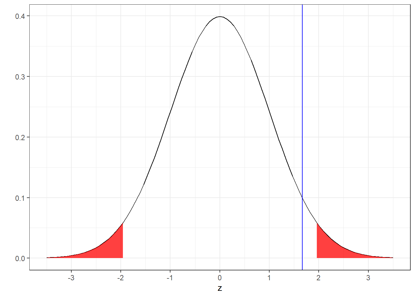
You can see that splitting the area of \(\alpha = 0.05\) into two halves increased the critical value in the positive direction from 1.64 to 1.96, making it harder to reject \(H_{0}\). For our example, this changes our decision: our observed value of z = 1.67 no longer falls into the rejection region, so now we fail to reject \(H_{0}\).
If we now fail to reject \(H_{0}\), what about the p-value? Remember, for a one-tailed test, p = \(\alpha\) if our observed z-score lands right on the critical value of z. The same is true for a two-tailed test. But the z-score moved so that the area above that score is \(\frac{\alpha}{2}\). So for a two-tailed test, in order to have a p-value of \(\alpha\) when our z-score lands right on the critical value, we need to double p-value hat we’d get for a one-tailed test.
For our example, the p-value for the one tailed test was \(p=0.0478\). So if we use a two-tailed test, our p-value is \((2)(0.0478) = 0.0956\). This value is greater than \(\alpha\) = 0.05, which makes sense because we just showed above that we fail to reject \(H_{0}\) with a two tailed test.
Which is the right test, one-tailed or two-tailed? Ideally, as scientists, we should be agnostic about the results of our experiment. But in reality, we all know that the results are more interesting if they are statistically significant. So you can imagine that for this example, given a choice between one and two-tailed, we’d choose a one-tailed test so that we can reject \(H_{0}\).
There are two problems with this. First, we should never adjust our choice of hypothesis test after we observe the data. That would be an example of ‘p-hacking’, a topic we’ll discuss later. Second, most statisticians these days strongly recommend against one-tailed tests. The only reason for a one-tailed test is if there is no logical or physical possibility for a population mean to fall below the null hypothesis mean.