28 Everything is normal: generating \(\chi^2\), \(F\) and \(t\) from z-scores

Remember that normal distributions can be generated by averaging draws from any distribution, thanks to the Central Limit Theorem. So the normal distribution shows up everywhere that things are summed or averaged. But the normal distribution is just one of several distributions we’ve covered in this class. It turns out that all of these other distributions are intimately related to the normal distribution.

This bonus chapter demonstrates how the three probability distributions that we’ve used for hypothesis testing in this class (\(t\), \(\chi^2\) and \(F\)) can be generated by manipulating draws from the standard normal (z) distribution. The point of this chapter is to show that these distributions are all related - and that tables and software giving probabilities associated with these distributions aren’t coming out of nowhere.

28.0.1 Means are normally distributed

Thanks to the Central Limit Theorem, the distribution of means from a population tend toward a normal distribution, even if the population is not normal. Thinking in terms of variances, if the population has mean \(\mu_x\) and standard deviation \(\sigma_x\), then the mean of the distribution of means (called the sampling distribution of the mean) is just the mean of the population:

\[\mu_{\bar{x}} = \mu_x\] And the variance of the sampling distribution of the mean is equal to the variance of the population divided by the sample size for each mean:

\[\sigma^{2}_{\bar{x}} = \frac{\sigma^{2}_{x}}{n} \]

For example, a uniform distribution that has equal probability between \(a\) and \(b\) will have mean: \(\frac{a+b}{2}\) and variance \(\frac{(a-b)^2}{12}\).

A uniform distribution with values ranging from \(-\sqrt{3n}\) to \(\sqrt{3n}\) will therefore have a mean of zero and a variance of \(\frac{(2\sqrt{3n})^2}{12} = n\).

This chunk of code generates a matrix with nSamples rows and n columns of values drawn from this distribution:

nSamples <- 100000
n <- 10

u <- matrix(runif(nSamples*n,-sqrt(3*n),sqrt(3*n)),ncol = n)

Here’s a histogram of the entire set of numbers with the expected uniform distribution drawn with it (in blue:). The verifies that the function runif is generating samples as expected.

Since the variance of this distribution is \(n\), the variance of the mean will be \(\frac{n}{n} = 1\). So thanks to the Central Limit Theorem, the means drawn from this distribution should look like the z-distribution (mean 0, standard deviation 1)

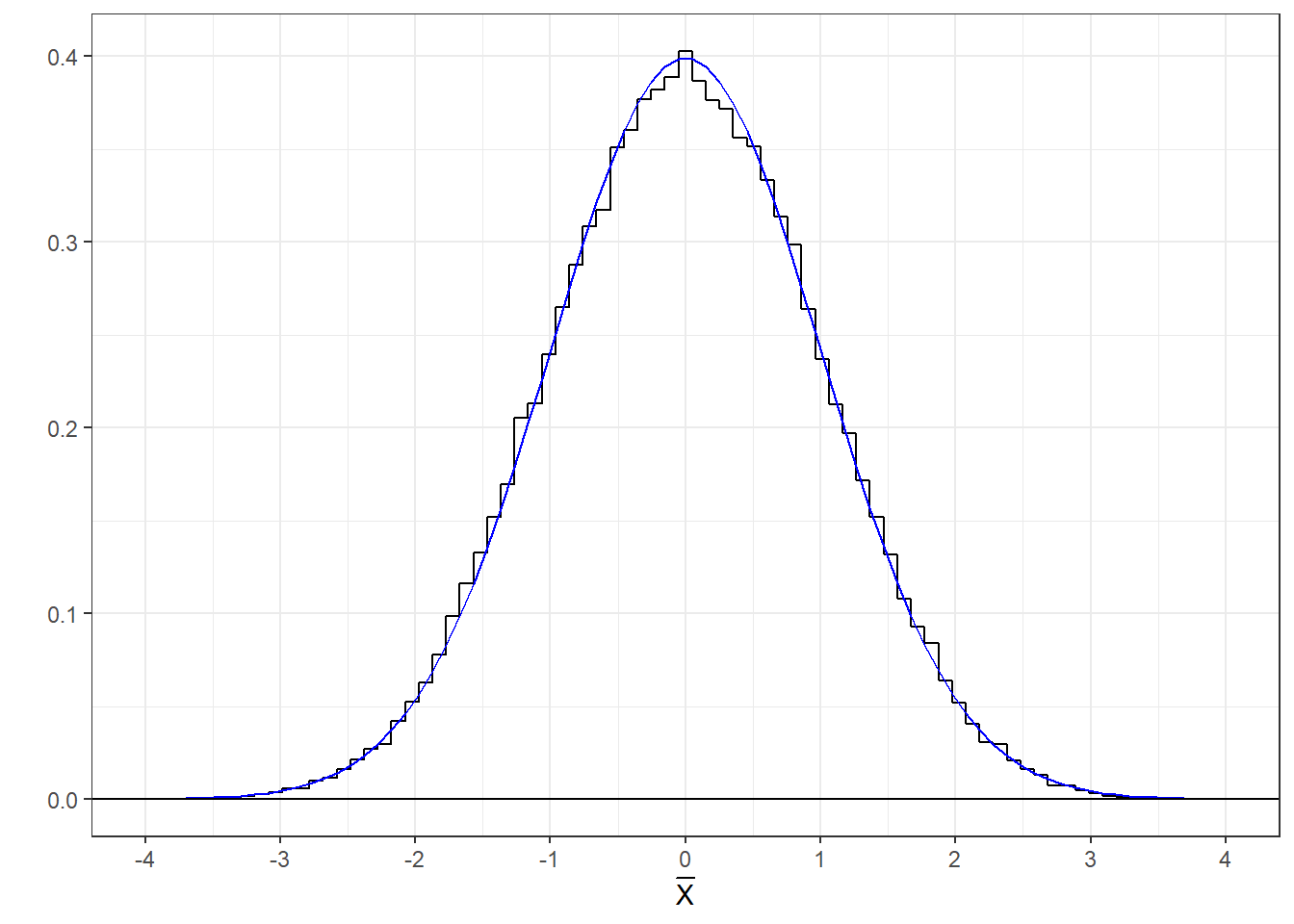
This calculates the mean of each row, which the mean of 10 samples from this uniform distribution:

uvar <- apply(u,1,var)
norm <- rowSums(u)/n 

Here’s a histogram of those means with the standard normal (z) distribution drawn with it. It matches well.

The mean from any population with variance \(n\) and mean 0 will be distributed like a z-distribution. The closer the population is to normality, and the larger the n, the more normal the distribution of means.

For the rest of this chapter we’ll just draw from the z-distribution using rnrorm to simulate other distributions. But keep in mind we could always start by drawing means from any distribution as long as it has a variance of \(n\) and mean 0.

28.0.2 The z-distribution

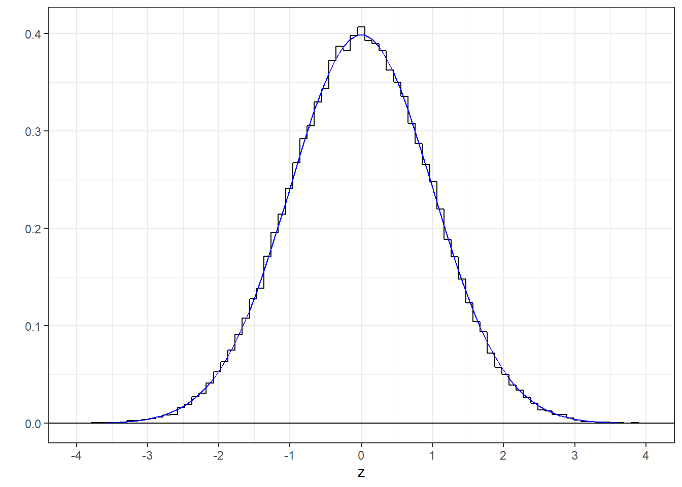
Let’s verify that a histogram of values drawn from rnorm match the probability distribution for z. Using ‘rnorm’ to sample from the standard normal distribution.

z <- rnorm(nSamples)

Here’s a histogram of these z-scores with the standard normal pdf drawn with it (using dnorm)

28.0.3 The \(\chi^2\) distribution

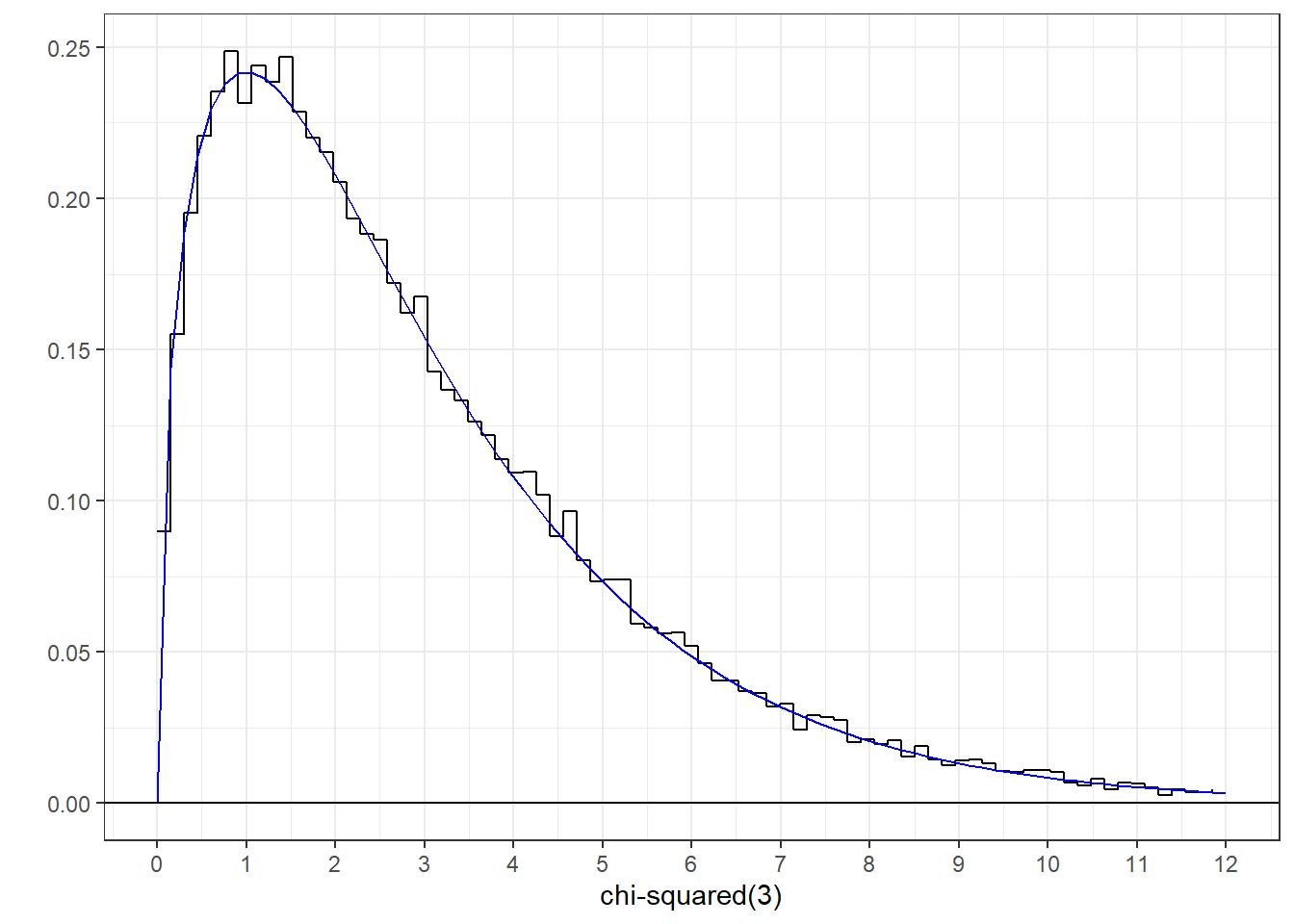
The \(\chi^2\) distribution can be generated by drawing \(df\) values from the z-distribution, squaring them and adding them up:

nSamples <- 30000
df <- 3

z <- matrix(rnorm(nSamples*df),ncol = df)
chi2 <- rowSums(z^2)  

Here’s a histogram of these simulated values with the \(\chi^2\) distribution of df = 3 drawn with it:

28.0.4 The distribution of variances

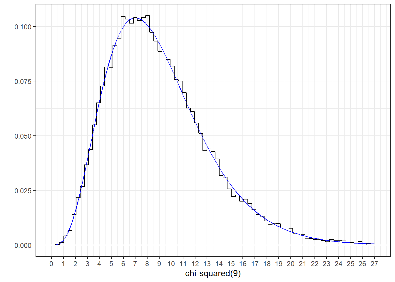
Variances of samples drawn from the z-distribution are distributed as \(\chi^2\) distributions with \(df = n-1\), divided by \(df\). Equivalently, the variance of n values from the z-distribution times \(df\) is equal to the \(\chi^2\) distribution.

This calculates a list of length nSamples, each is the variance of n values drawn from the z distribution, multiplied by \(df = n-1\):

n <- 10
df <- n-1

z <- matrix(rnorm(nSamples*n),ncol = n)
dftimesvar <- df*apply(z,1,var)

Here’s a histogram of these values with the \(\chi^2\) distribution of degree 9 drawn with it.

28.0.5 The F distribution

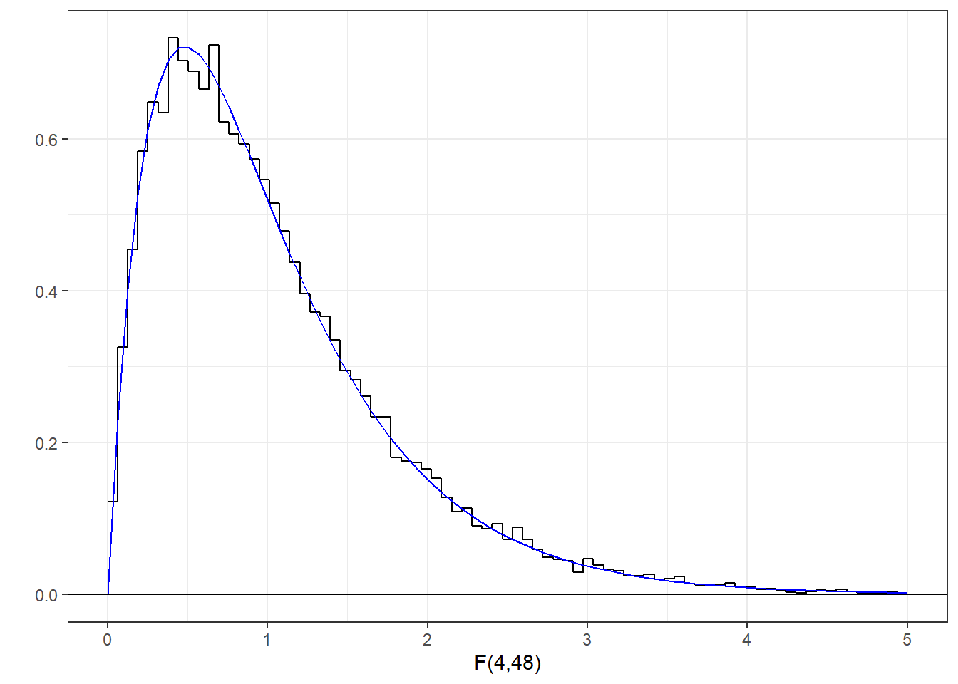
The \(F\) distribution is the ratio of two \(\chi^2\) distributions, each divided by their degrees of freedom. \(F\) is therefore the ratio of two variances (hence ‘ANOVA’). Since \(\chi^2\) distributions can be generated from squared z-scores, it all starts with the z-distribution. This generates the ratio of two \(\chi^2\) distributions, each divided by their degrees of freedom:

df1 <- 4
df2 <-48

z1 <- matrix(rnorm(nSamples*df1),ncol = df1)  # To generate numerator chi-square
z2 <- matrix(rnorm(nSamples*df2),ncol = df2)  # To generate denominator chi-square
Fsim <- (rowSums(z1^2)/df1)/(rowSums(z2^2)/df2)  

Here’s a histogram of these values with the F-distribution having 4 and 48 degrees of freedom drawn with it:

28.0.6 The t-distribution

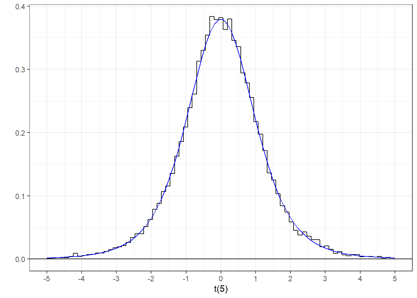
The t-distribution is the ratio of a z-distribution divided by a distribution of standard deviations. Since variances are distributed as \(\chi^2\) divided by \(df\), standard deviations are its square root. Again, the t-distribution can be generated by manipulating draws from the standard normal:

df <- 5

z1 <- rnorm(nSamples)
z2 <- matrix(rnorm(nSamples*df),ncol = df)

tsim <- z1/(sqrt(rowSums(z2^2)/df))  

Here’s a histogram of our values with the t-distribution with df = 5 drawn with it:

So that’s it. I should point out that one other distribution that we’ve used, the binomial distribution, isn’t directly generated by normal distributions but can be closely approximated by it. So the binomial distribution gets honorable mention in this chapter.

These simulations aren’t particularly useful for solving statistical inference problems, but I hope they relieve some of the mystery behind the origins of the \(\chi^2\), \(F\), and \(t\) distributions.

28.0.7 List of parametric distributions

R \(p\), \(q\), \(r\), and \(d\) versions of a huge number of parametric distributions. Most, but not all of them can be derived from various manipulations of the standard normal (z) distribution. Here’s a current list, many of these have been covered in this book:

Table 28.1:

	p	q	d	r
Beta	pbeta	qbeta	dbeta	rbeta
Binomial	pbinom	qbinom	dbinom	rbinom
Cauchy	pcauchy	qcauchy	dcauchy	rcauchy
Chi-Square	pchisq	qchisq	dchisq	rchisq
Exponential	pexp	qexp	dexp	rexp
F	pf	qf	df	rf
Gamma	pgamma	qgamma	dgamma	rgamma
Geometric	pgeom	qgeom	dgeom	rgeom
Hypergeometric	phyper	qhyper	dhyper	rhyper
Logistic	plogis	qlogis	dlogis	rlogis
Log Normal	plnorm	qlnorm	dlnorm	rlnorm
Negative Binomial	pnbinom	qnbinom	dnbinom	rnbinom
Normal	pnorm	qnorm	dnorm	rnorm
Poisson	ppois	qpois	dpois	rpois
Student t	pt	qt	dt	rt
Studentized Range	ptukey	qtukey	dtukey	rtukey
Uniform	punif	qunif	dunif	runif
Weibull	pweibull	qweibull	dweibull	rweibull
Wilcoxon Rank Sum Statistic	pwilcox	qwilcox	dwilcox	rwilcox
Wilcoxon Signed Rank Statistic	psignrank	qsignrank	dsignrank	rsignrank