Chapter 26 Nonparametric Tests
Up to now all of the statistical tests we’ve done have involved calculating a statistic that we can look up in a table. These are parametric tests, because if the data satisfy assumptions such as normality, homogeneity of variance and sphericity, then we can assume that the computed statistic will be drawn from a known, parametric distribution such as a t, F, or \(\chi^{2}\). If you can’t assume that your data satisfies the conditions of a parametric test you can run a nonparametric test.
Some of the nonparametric tests discussed in this tutorial are direct alternatives to parametric tests that we’ve covered in this class. Here’s our familiar flow-chart:

The four tests in purple boxes are some of the tests we’ll cover in this chapter Each of these four has a corresponding parametric test above it in the flow chart. For example the ‘Friedman’s rank test’ is a direct substitute for the repeated measures ANOVA. This chapter walks through some of the standard nonparametric tests. It also covers alternatives such as bootstrapping, resampling and rank transformations.
26.1 Example: RT for recognizing famous faces
Suppose we’re interested in how experience affects the ability to recognize celebrity faces. We ask 8 experts and 12 novices to identify famous faces and measure their response times.
You can load in the (fake) data set here:
Here are the response times (in seconds), with experts colored in green and novices colored in blue:
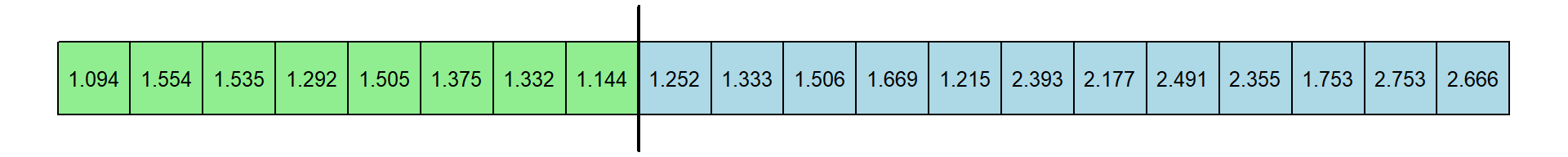
It’s hard to tell from the raw numbers which group has a larger central tendency. Here’s how to plot at a histogram of the two distributions:
ggplot(dat = dat1, aes(x = RT,fill = condition,col = condition)) +
  geom_histogram(position="dodge2", alpha=.8,breaks = seq(1,max(dat1$RT)+.1,by = .1))+
  scale_fill_manual(values=col)+
  scale_color_manual(values=col)+
  xlab("Response Time (sec)") + ylab("Frequency") +
  theme_bw()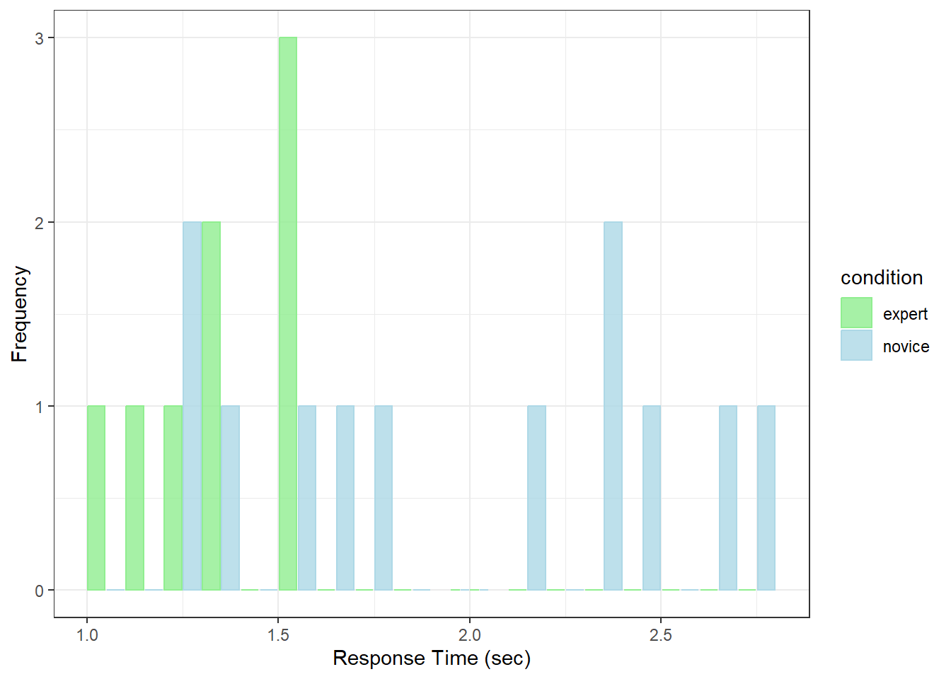
It looks like the novices are slower.
Response times distributions are often positively skewed like this, so the median may be a better estimate of central tendency. This means that all of our statistics on means do not apply - so we can’t use our standard independent measures t-test here.
In fact, a Shapiro-Wilk test will not reject the hypothesis test that these distributions came from a normal population. This is probably because our sample size is so small - so the test for normality is under powered. This is a good example of why we should be careful about ‘accepting the null hypothesis’ when a result is not statistically significant. I happen to know that the populations that these samples were drawn from non-normal distributions because I made the data up by sampling from shifted and scaled \(\chi^{2}\) distributions with \(df = 3\).
The medians are:
## expert novice
## 1.3535 1.9650The difference between these medians is 0.6115 seconds. We’d like determine if this difference is significantly different from zero.
26.2 The Permutation Test
How can we calculate a p-value for this observed difference in medians? We’ll start with a permuation test. Permutation simulations involve exchanging labels on data points to get an estimate of the sampling distribution under the null hypothesis. Permutation tests also go by the names of exact tests, randomization tests, or re-randomization tests.
Our null hypothesis is that the two samples of RT’s are drawn from the same population (or two identical populations). This means that for our sample of 20 RTs there is nothing special about first 8 being drawn from the experts group the remaining 12 being drawn the from novice group. That is, the difference in medians that we observed shouldn’t be any more extreme than for any arbitrary reordering of the samples.
For example, let’s reorder our 20 samples using the sample function:
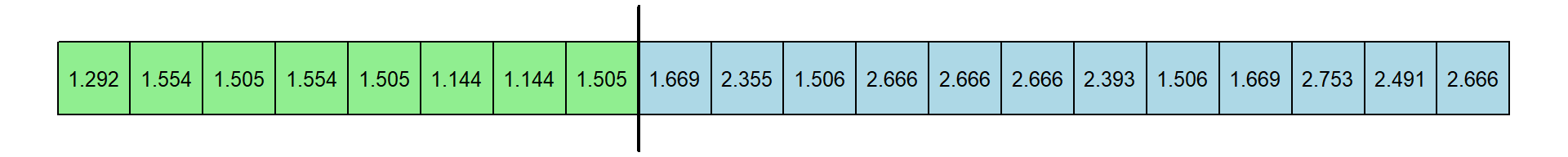
Here’s a new table of RT’s. I’ve kept the original color coding. Let’s pretend that the first 8 came from experts, indicated by the vertical line:
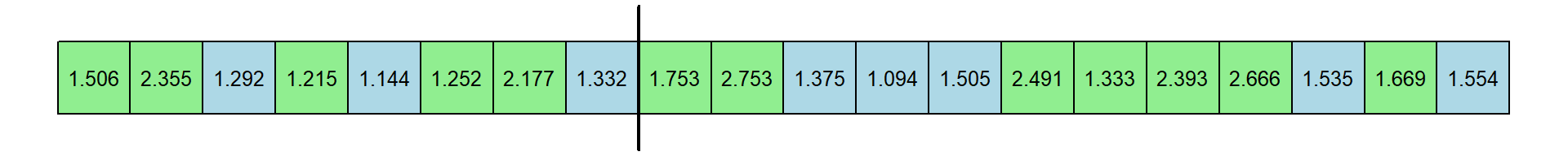
The median of the first 8 response times is 1.312 and the median of the remaning 12 response times is 1.6115. The new differences is 0.2995 seconds. This is just one permutation. Here’s another:
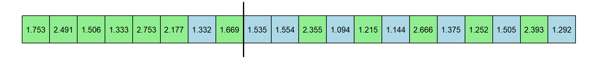
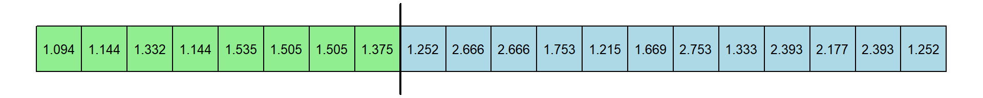
Now the median of the first 8 response times is 1.711 and the median of the remaning 12 response times is 1.44. This differences is -0.271 seconds.
Permutation tests involve calculating our statistic on many, many permutations and see how unusual our observed statistic is compared to the statistics from the resampled data sets. You can think of the distribution of resampled statistics as our estimate of the population distribution of the null hypothesis, which is that there isn’t anything special about how our 20 RT’s are divided into the two categories.
Our p-value will be the proportion of resampled medians that are more extreme than our observed statistic.
The following chunk of R code repeatedly permutes the RT’s and recalculates the differences between the median of the first 8 RTs and the median of the last 12 RTs:
nReps <- 10000
permute.median.diff <-  matrix(data=NA,ncol=nReps)
for (i in 1:nReps) {
  # 'sample' by default samples without replacement, which is a permutation
  permute.RT <- sample(dat1$RT)
  # calculate the median RT's for this permuted data
  # using the 'condition' coding from the real data:
  medians <- tapply(permute.RT,dat1$condition,median)
  # save the difference in medians for this permutation
  permute.median.diff[i] <- diff(medians)
}
Here’s a histogram of the differences in medians for these 10000 permutations.
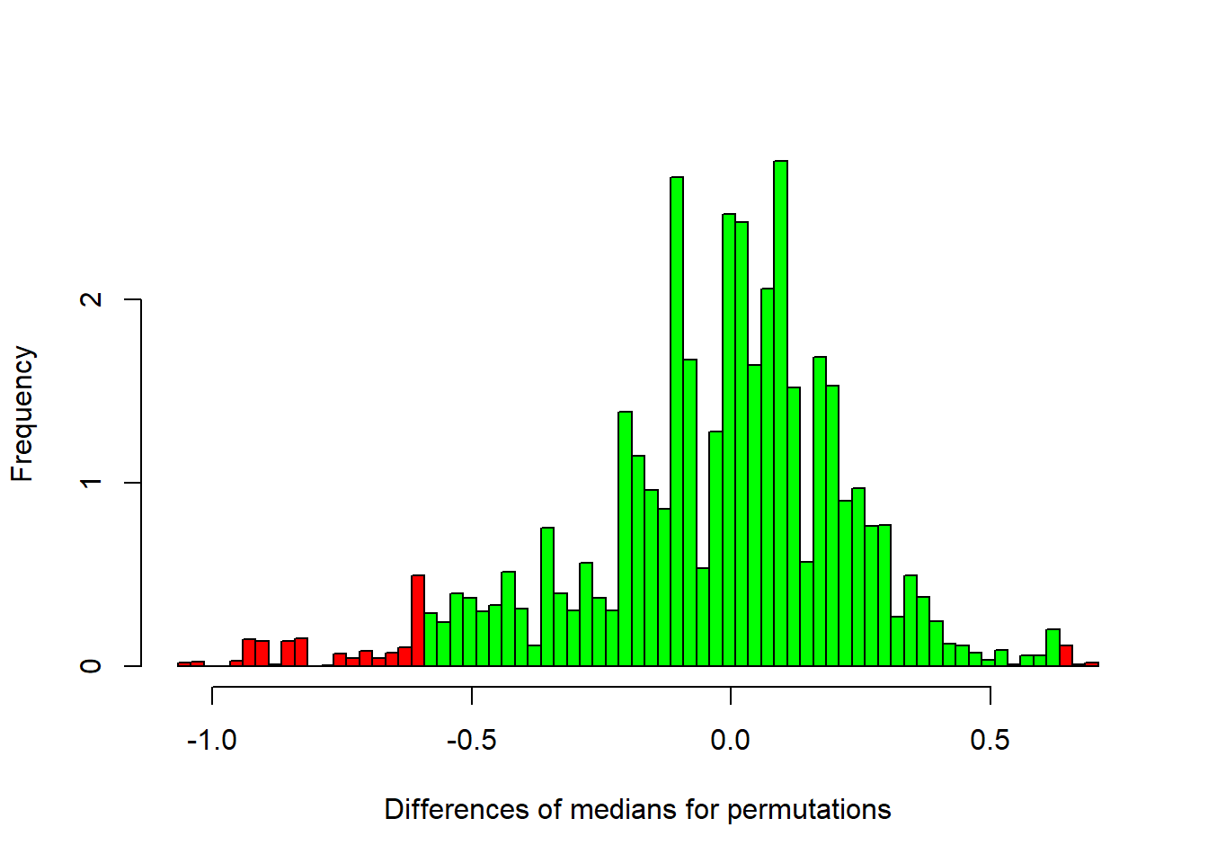
I’ve colored in red the permutations that generated differences in medians that are more extreme (in absolute value) than our observed difference of +/- 0.6115. The remaining are in green.
This is a complicated looking distribution, but it’s our best guess at the sampling distribution of median differences under the null hypothesis.
Now all we do is calculate the proportion of these permutations that fell into the red zones. This serves as a p-value for the permutation test:
permute.p.value <- sum(abs(permute.median.diff) > abs(diffObserved))/nReps
sprintf('Permutation test p = %5.4f ',permute.p.value)
## [1] "Permutation test p = 0.0371 "The proportion of differences that are colored red is 0.0371. This serves as our p-value. If this value is less than \(\alpha\) = 0.05 we should reject \(H_{0}\) and conclude that there is a significant difference in medians between the two groups.
26.3 Bootstrapping - sampling with replacement
We can use another kind of resampling method called bootstrapping to estimate the likelihood of our observed statistic. Bootstrapping methods involve generating fake data sets based on your observed data and re-running your statistic. Fake data sets are obtained by sampling with replacement your observed data. The idea is that these resampled data sets reflect the statistical properties of your sample, and therefore the properties of the population they came from. For this example, we’ll generate 8 fake RT’s for the expert group by resampling with replacement the original 8 RT’s, and do the same for the 12 RT’s for the novice group:
Here’s a nice use of tapply to resample RT’s for each level of condition.
f <- function(x) sample(x,length(x),replace = TRUE)
resample.out <-   tapply(dat1$RT,dat1$condition,f)
Here’s the resampled data:
Now the median of the 8 resampled expert response times is 1.505 and the median of the 12 resampled novice response times is 2.442. This differences is 0.937 seconds.
Here’s another one:
For this resampled data set, the median expert response times is 1.3535 and the median of novice response times is 1.965. This differences is 0.6115 seconds.
Sampling with replacement means that some RT’s will be sampled more than once, and others will be left out. It turns out that resampled data like this is good way of generating new data sets that have the same statistical properties (means, standard deviations, skewness…) as the population that the original data set was drawn from.
After resampling we recalculate our statistic, which is the absolute value of the difference between medians. On average the resampled statistic will tend toward the statistic from the original data. But it will vary each time we resample, and it’s this variability that we use to estimate the likelihood of our observed statistic.
Unlike for the permutation test, were the differences in medians averages around zero, the typical difference in medians for a resampled data set is expected to be somewhere around differences in the medians for the real data set.
The following chunk of R code continues this resampling process, generating a distribution of differences of medians:
nReps <- 10000
bootstrap.median.diff <-  matrix(data=NA,ncol=nReps)
f <- function(x) sample(x,length(x),replace = TRUE)
for (i in 1:nReps) {
  resample.out <-   tapply(dat1$RT,dat1$condition,f)
  bootstrap.median.diff[i] <-
    median(resample.out$novice) -
    median(resample.out$expert)
}
Here’s a histogram of the resampled differences of medians:
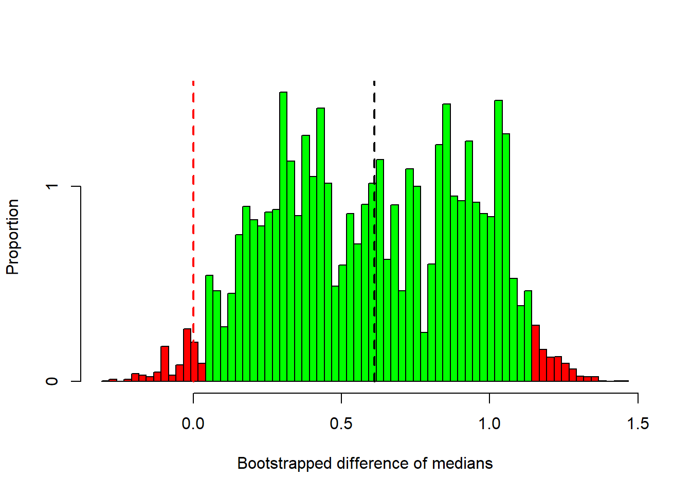
This histogram is our guess at what the population distribution looks like for the difference between medians. Remember, our observed median is was 0.6115, which I’ve indicated with a dashed black line. It’s right in the middle of the distribution, but you can see that some of differences after resampling can be quite far away from our observed difference.
I’ve colored in green the bootstrapped statistics that fall within the middle 95 and red outside. These green samples fall within the 95 confidence interval. These values are:
##   2.5%  97.5%
## 0.0410 1.1385
We reject \(H_{0}\) if the confidence interval does not contain the value for the null hypothesis (which is zero in our case).
This confidence interval does not contain zero (the green bars don’t reach the red dashed line). This means that differences in the medians of our resampled data fall below zero less than 2.5 of the time. We therefore conclude that our observed difference of medians is significantly different from zero using an alpha value of \(\alpha\) = 0.05.
We can also calculate a p-value from the bootstrapped medians. This is the proportion of resampled differences that fall below zero, multiplied by two to get a two-tailed test:
## [1] 0.0386This is just the tip of the iceberg for how bootstrapping works. Formally, we should be using a modification of this procedure that corrects for a bias with small samples. There are various ways proposed to do this. The most common is the bias-corrected and accellerated (BCa) method. For proper implementation, R has a package that does all the resampling and bias correction called boot.
26.4 Statistics on ranks
We now move onto the more traditional nonparametric tests, seen in the purple boxes in the flow chart above. All of these tests involve ‘rank transformations’ of the data in some way or another. Rank transformations simply replace the observations in a sample by their corresponding ranks starting with 1 as the lowest observation.
The ranks of a list have a known mean and standard deviation. A list of numbers counting from 1 to n has a sum of
\[\frac{n(n+1)}{2}\]
and therefore a mean of
\[\frac{n+1}{2}\]
and a (population) variance of
\[\frac{n^{2}-1}{12}\] A rank transformation a set of n numbers will always have this mean and standard deviation since the order of the values don’t matter.
Nonparametric tests that use rank transformations use these known means and transformations to calculate p-values. For example, if you have a data set with two groups of equal size and you rank order the entire set of numbers, then under the null hypothesis, we’d expect half of the ranks to fall randomly into each set. The sum of an arbitrary half of the ranks will therefore be, on average, half of the sum of all of the ranks:
\[\frac{n(n+1)}{4}\]
But the variance of an arbitrary half of ranks should, on average, be the same as the variance of all of the ranks. So now we have two means and variances which can be used to calculate a p-value. Note that the formula for the standard deviation above leads to strange constants like 4 and 12 in some of the equations for nonparametric tests that use ranks.
26.4.1 Dealing with ties
A note about ties: when ranking a list of numbers, if there are repeated values (ties) then the ranks for all of those ties are given the same number - the mean of the ranks that they’d have if they weren’t ties. You can see how R does with the rank function for a list with ties:
## [1] 1.0 2.5 2.5 4.0 5.0The second and third in the list are ties. So they each get a rank of 2.5. Ties mess up the expected means and standard deviations of a rank transformation a bit. Sometimes this is ignored. R’s nonparametric test functions will give you scary warnings and run normal approximation versions of the tests instead, which we’ll cover below.
26.5 Wilcoxon’s Rank-Sum Test
One well-known test that uses rank transformations is the Wilcoxon’s Rank-Sum test which is the nonparametric alternative to the independent measures t-test. It tests the null hypothesis that two medians from two samples came from the same population. The Wilcoxson’s Rank Sum is the same as the Mann-Whitney U test. Both give the same p-values, though with slightly different statistics (W for Wilcoxon and R for Mann-Whitney).
Later on we will introduce the Kruskal-Wallis nonparametric test which works for more than two independent means. Just like the 1-way ANOVA is a generalization of the two sample t-test, the Kruskal-Wallis is a generalization of the Wilcoxon’s Rank-Sum Test. The Kruskal-Wallis test is actually a lot easier to implement than the Wilcoxon test. I’ll say it here - we don’t need the Wilcoxon’s Rank-Sum Test, but I’m covering it because it is a common test that you’ll see in the literature.
26.5.1 The procedure:
The procedure works by giving ranks for each of the 20 response times. Here is the original set of RT’s and the rank transformation:

You should appreciate that if the experts have shorter RTs then the ranks for these 8 RTs should be smaller than for the novices. You should also appreciate that these ranks, like medians, are not dependent on the actual value of the extreme values - just their relative order.
The dependent measure in the Wilcoxon’s Rank Sum test starts with adding up the ranks for each of the two groups:
For experts: \(1+12+11+5+9+8+6+2 = 54\)
for the novices: \(4+7+10+13+3+17+15+18+16+14+20+19 = 156\)
We then calculate \(W_{1}\) and \(W_{2}\) by subtracting the minimum value possible: \(\frac{(n)(n+1)}{2}\), where \(n\) is the sample size for that group
\(W_{1} = R_{1} -\frac{n_{1}(n_{1}+1)}{2}\)
\(W_{2} = R_{2}-\frac{n_{2}(n_{2}+1)}{2}\)
For our example:
(expert) \(W_{1} = 54 - \frac{(8)(9)}{2} = 18\)
(novice) \(W_{2} = 156 - \frac{(12)(13)}{2} = 78\)
The W’s have a known distribution. R has it’s own function pwilcox that will convert your observed value of \(W\) to a p-value. Assuming a two-tailed test:
## [1] 0.02013178Note that sometimes, the values of \(R_{1}\) and \(R_{2}\) are used instead of \(W_{1}\) and \(W_{2}\). By default, R gives you the smaller of the two values of W.
26.5.2 Using R:
Here’s how to run the Wilcoxon rank sum test in R and how to organize the results into an APA format. The ‘formula’ RT ~ condition is the way we define the independent and dependent variables in lm:
wrs.out.exact <- wilcox.test(RT ~ condition,data = dat1,exact = TRUE)
sprintf('W = %g, p = %5.4f',wrs.out.exact$statistic,wrs.out.exact$p.value)
## [1] "W = 18, p = 0.0201"You might notice that the p-value we get from the Wilcoxon Rank Sum test is not the same as the permutation test (0.0371). I’ve found with simulations that under the null hypothesis the correlation between the two p-values is only about 0.75.
Technically this is the ‘Exact’ version of the Wilcoxon’s rank-sum test, hence the exact = TRUE input.
26.6 Wilcoxon’s Rank Sum Test: The Normal Approximation
R has trouble with the exact test when there are ties. Also, calculating the p-values for \(W\) (e.g. with pwilcox) can take up a large amount of time and computer memory if the sample sizes are large. If either there are ties or the sample sizes are large, R will run the inexact version automatically.
When you set exact=FALSE with wilcox.test, the test uses a normal approximation to the distribution of \(W\) based on the the means and standard deviations of ranks discussed earlier. Here’s how it works:
26.6.1 The procedure:
For larger sample sizes (the rule is a total of about 25 observations) the distribution of the smallest of the two summed ranks tends toward a normal distribution that has a mean of:
\[\mu = \frac{n_1(n_1+n_2+1)}{2}\]
And a standard deviation:
\[\sigma = \sqrt{\frac{n_1 n_2(n_1+n_2+1)}{12}}\]
For our example:
\[\mu = \frac{8(21)}{2} = 84\] \[\sigma = \sqrt{\frac{(8)(12)(21)}{12}} = 12.9615\]
26.6.2 By hand:
We can use pnorm to calculate the probability of obtaining a value of R drawn from a normal distribution with these means and standard deviations. Here’s (presumably) how R computes the normal approximation to the Wilcoxon’s rank sum test:
# calculate the sample sizes, sum of ranks and R (the smallest sum of ranks)
n <-  tapply(ranked.dat1$RT,ranked.dat1$condition,length)
sumRanks <- tapply(ranked.dat1$RT,ranked.dat1$condition,sum)
R <- min(sumRanks)
# calculate the mean and standard deviation of normal approximation to R for H0
mu <- as.numeric(n[1]*(n[1]+n[2]+1)/2)
sigma <- as.numeric(sqrt(n[1]*n[2]*(n[1]+n[2]+1)/12))
# use pnorm to get the p-value based on R - using correction for continuity (two-tailed)
p <- 2*(pnorm(R+.5,mu,sigma))
sprintf('p = %5.4f',p)
## [1] "p = 0.0228"26.6.3 Using R:
Here’s how to run the ‘nonexact’ version of the test by setting exact = FALSE:
wrs.out.exact <- wilcox.test(RT ~ condition,data = dat1,exact = FALSE)
sprintf('W = %g, p = %5.4f',wrs.out.exact$statistic,wrs.out.exact$p.value)
## [1] "W = 18, p = 0.0228"The p-value matches the value we calculated by hand.
26.7 Wilcoxon’s Matched-Pairs Signed-Ranks Test
The Wilcoxon Matched-Pairs test is a nonparametric alternative to the dependent-measures t-test.
Suppose now that you want to study the ability to recognize famous faces at a distance (Geoff Loftus was doing this experiment outside my office, using our long hallway as a laboratory) You find 10 subjects and ask each to identify famous faces from a near and far distance.
Here’s how to load in the data:
26.7.1 The procedure:
The first two columns in the following table is our list of response times:
| one meter | 10 meters | \(D\) | \(|D|\) | Rank of \(|D|\) | |
|---|---|---|---|---|---|
| S1 | 1.539 | 2.849 | -1.310 | 1.310 | 9 |
| S2 | 2.207 | 4.049 | -1.842 | 1.842 | 10 |
| S3 | 1.359 | 2.552 | -1.193 | 1.193 | 7 |
| S4 | 3.725 | 3.902 | -0.177 | 0.177 | 2 |
| S5 | 3.025 | 3.408 | -0.383 | 0.383 | 5 |
| S6 | 3.298 | 3.375 | -0.077 | 0.077 | 1 |
| S7 | 5.360 | 5.025 | 0.335 | 0.335 | 4 |
| S8 | 4.213 | 3.898 | 0.315 | 0.315 | 3 |
| S9 | 2.003 | 3.297 | -1.294 | 1.294 | 8 |
| S10 | 1.377 | 2.055 | -0.678 | 0.678 | 6 |
The third column is the difference between conditions, \(D\), just as we would calculate for the repeated measures t-test. Notice that 2 of the 10 differences are positive.
The Wilcoxon’s Matched-Pairs Signed-Ranks Test is based on a ranking of the absolute value of these differences. Absolute values are in the fourth column and corresponding ranks of the absolute values of D are in the fifth column.
Zeros values of \(D\) are ignored, so the first positive value is given a rank of 1 and so on.
I’ve colored the rows for the positive differences in green, and the negative differences in red. You can see visually the balance between the two. Our statistic, called \(V\) is the sum of the ranks for rows with positive differences, which is 7:
\(V\) = \(4+3 = 7\)
)Like \(W\), the distribution for \(V\) under the null hypothesis can be calculated. The gist is that with the null hypothesis, half of the ranks should contribute to \(V\) on average. Earlier we showed that the average of half the ranks is \(\frac{n(n+1)}{4} = 27.5\). We reject \(H_{0}\) if \(V\) gets too far away from this value.
R has it’s own function psignrank that will calculate a p-value from your observed value of V:
## [1] 0.0371093826.7.2 Using R:
We use wilcox.test again to run this test but this time we’ll set paired = T Here’s how it’s done:
x <- dat2$RT[dat2$condition == 'one_meter']
y <- dat2$RT[dat2$condition == 'ten_meters']


wp2.out <- wilcox.test(x,y,exact = T,paired = T)
sprintf('Wilcoxon Matched Pair Sign Rank Test: V = %g, p = %5.4f ',
        wp2.out$statistic,wp2.out$p.value)
## [1] "Wilcoxon Matched Pair Sign Rank Test: V = 7, p = 0.0371 "26.8 Wilcoxon’s Matched-Pairs Signed-Ranks Test n>50: The Normal Approximation
Just like for the Wilcoxon Ranked-Sum Test, there is a normal approximation for larger number of pairs (typically greater than 50). Note: I’ve seen examples of the normal approximation used for only 10 or more pairs (e.g. https://en.wikipedia.org/wiki/Wilcoxon_signed-rank_test). Like for the Wilcoxon’s rank sum test, calculating the distribution of V for large samples can be very time consuming, so R will switch to the normal approximation for a large sample size.
26.8.1 The procedure:
The mean of this distribution of T’s is:
\[\mu = \frac{n(n+1)}{4}\]
And the standard deviation is:
\[\sigma = \sqrt{\frac{n(n+1)(2n+1)}{24}}\]
For our example (even though our sample size is less than 50)
\[\mu = \frac{10(11)}{4} = 27.5\]
and
\[\sigma = \sqrt{\frac{10(11)(21)}{24}} = 9.8107\]
26.8.2 By hand:
We can use R’s pnorm function to find the probability of obtaining a value of V= 7 or more extreme when drawn from a normal distribution with these mean and standard deviations. Here’s how to do it by hand. Note the calculation of the z-score - abs(V-mu)-.5) is a way of doing the correction for continuity, regardless of whether V is greater or less than \(\mu\).
n <- 10
mu <- n*(n+1)/4
sigma <- sqrt(n*(n+1)*(2*n+1)/24)
z <- (abs(V-mu)-.5)/sigma
p <- 2*(1-pnorm(abs(z)))
sprintf('p = %5.4f',p)
## [1] "p = 0.0415"26.8.3 Using R:
You can run the ‘inexact’ version of the Wilcoxon’s matched-pairs signed-ranks test like this:
x <- dat2$RT[dat2$condition == 'one_meter']
y <- dat2$RT[dat2$condition == 'ten_meters']


wp2.out <- wilcox.test(x,y,paired = TRUE,exact=FALSE)
sprintf('Wilcoxon Matched Pair Sign Rank Test (inexact): V = %g, p = %5.4f ',
        wp2.out$statistic,wp2.out$p.value)
## [1] "Wilcoxon Matched Pair Sign Rank Test (inexact): V = 7, p = 0.0415 "The p-values match what we calculated by hand.
26.9 Sign Test
Another nonparametric test that we can used for dependent-measures samples is the Sign Test. We look at the number of positive and negative values of D to see how likely this could happen by chance using the binomial distribution with P= .5. For our example, we want to calculate the probability of getting 8 out of 20 (or more) positive differences. This is really just a binomial test on the number of positive differences (see section 12.6)
26.9.1 Using R:
This can be done simply with binom.test, after counting the number of positive differences.
# count the number of positive differences
k <- sum(dat2$RT[dat2$condition=="ten_meters"]  > dat2$RT[dat2$condition=="one_meter"] )
n <- sum(dat2$condition=="one_meter")
sign.out <- binom.test(k,n,.5,alternative = 'two.sided')
sprintf('Sign test: k = %d, n = %d, p = %5.4f',
        sign.out$statistic,sign.out$parameter,sign.out$p.value)
## [1] "Sign test: k = 8, n = 10, p = 0.1094"The sign test is the nonparametric test that uses the least amount of information in our data. It makes the fewest assumptions about how our data is distributed and is therefore the least powerful.
In the middle is the Wilcoxon’s Matched-Pairs Signed-Ranks test, which takes into account the order of the differences. The dependent measures t-test assumes the most, and is the most powerful, as long as the conditions are satisfied.
26.10 Normal approximation to the Sign Test
Remember the normal approximation to the binomial distribution? I bet you do (section 12.5). The Sign Test is just a binomial test, so for sample sizes of 20 or more we can use the normal approximation to the binomial. We have only 10 differences in our example, but we can work out The procedure anyway:
26.10.1 The procedure:
Remember, the expected number of positive differences under the null hypothesis has a mean of:
\[\mu = NP\]
And the standard deviation is:
\[\sigma = \sqrt{NP(1-P)} = \sqrt{N(.5)(.5)}\]
For our example
\[\mu = (10)(.5) = 5\] and
\[\sigma = \sqrt{10(.5)(.5)} = 1.58\]
26.10.2 By hand:
We can use pnorm to calculate the probability of getting 8 or more out of 10 positive differences (or more extreme). Here’s how to do it. Note the correction for continuity again:
# quick way to get a list of RT's by condition
dat_list <-tapply(dat2$RT,dat2$condition,rbind)
D <- dat_list$ten_meters - dat_list$one_meter
V <- sum(rank(abs(D))[D>0])
n <- length(dat_list$one_meter)
mu <- n*.5
sigma <- sqrt(n*.5*.5)

z <- (abs(k-mu)-.5)/sigma
p <- 2*(1-pnorm(abs(z)))
sprintf('p = %5.4f',p)
## [1] "p = 0.1138"This normal approximation is pretty close to the ‘exact’ result from the binomial test.
26.11 Kruskal-Wallis One-Way ANOVA
This is a nonparametric version of the independent measures ANOVA for cases where assumptions like normality and homogeneity of variance are violated. Like the Wilcoxon’s Rank-Sum Test, it relies on rank-ordering the data.
Let’s add one more group to our original study on recognizing famous faces for expert and novices and find 10 monkeys to participate in our study. You can load in the example data set like this:
The data set now looks like this:
| expert | novice | monkey |
|---|---|---|
| 1.094 | 1.252 | 1.343 |
| 1.554 | 1.333 | 1.463 |
| 1.535 | 1.506 | 1.623 |
| 1.292 | 1.669 | 1.720 |
| 1.505 | 1.215 | 1.365 |
| 1.375 | 2.393 | 2.571 |
| 1.332 | 2.177 | 1.493 |
| 1.144 | 2.491 | 2.922 |
| 2.355 | 2.527 | |
| 1.753 | 1.674 | |
| 2.753 | ||
| 2.666 |
Here’s a histogram with the new set of subjects:
ggplot(dat = dat3, aes(x = RT,fill = condition,col = condition)) +
  geom_histogram(position="dodge2", alpha=.8,breaks = seq(1,max(dat3$RT)+.1,by = .1))+
  scale_fill_manual(values=col)+
  scale_color_manual(values=col)+
  xlab("Response Time (sec)") + ylab("Frequency") +
  theme_bw()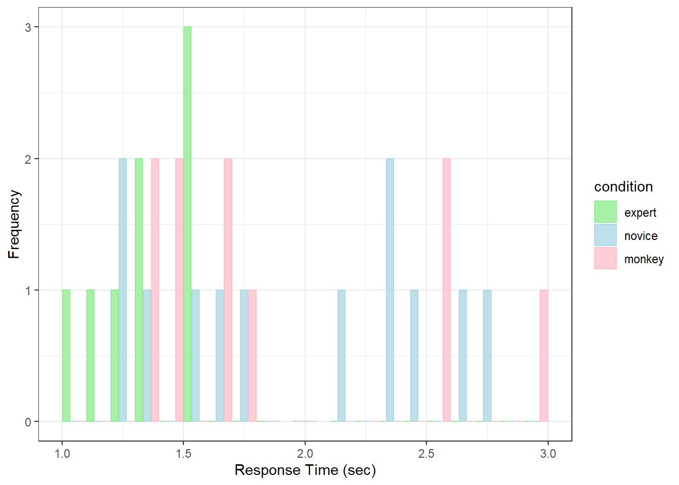
26.11.1 The procedure:
For the Kruskal-Wallis test we find the ranks for each of these RT’s as if they were all in one pile. Here’s the rank transformation:
| expert | novice | monkey |
|---|---|---|
| 1 | 4 | 8 |
| 16 | 7 | 11 |
| 15 | 14 | 17 |
| 5 | 18 | 20 |
| 13 | 3 | 9 |
| 10 | 24 | 27 |
| 6 | 22 | 12 |
| 2 | 25 | 30 |
| 23 | 26 | |
| 21 | 19 | |
| 29 | ||
| 28 |
The null hypothesis is that the average rank for each group is the same. The statistic we calculate to measure this is called ‘H’ which under th null hypothesis is approximated by a \(\chi^{2}\) distribution with k-1 degrees of freedom (k is the number of groups, 3 for our example).
First we calculate the sum of the ranks for each column. For our example:
For expert: \(R_{1}\) = \(1+16+15+5+13+10+6+2 = 68\)
For novice: \(R_{2}\) =\(4+7+14+18+3+24+22+25+23+21+29+28 = 218\)
For monkey: \(R_{3}\) =\(8+11+17+20+9+27+12+30+26+19 = 179\)
The statistic H is then calculated with this crazy formula:
\[H=\frac{12}{N(N+1)}(\sum{\frac{R_i^2}{n_i}})-3(N+1)\]
Where N is the total number of measurements (\(8+12+10 = 30\)).
For our example:
\[H = \frac{12}{30(31)}(578+3960.33+3204.1)-3(30+1)=6.9\]
26.11.2 By hand:
Here’s how to do this by hand:
R <- tapply(rank(dat3$RT),dat3$condition,sum)
n <- table(dat3$condition)
N <- sum(n)
H <- 12/(N*(N+1)) * (sum(R^2/n)) - 3*(N+1)
df = length(n)-1
p <- 1-pchisq(H,df)
sprintf('chi-squared(%d) = %5.4f, p = %5.4f',df,H,p)
## [1] "chi-squared(2) = 6.9024, p = 0.0317"26.12 Friedman’s Rank Test
Our final nonparametric test of the book (are you sad?) is the nonparametric version of the repeated measures 1-way ANOVA, the Friedman’s Rank Test. This is the same Milt Friedman, the U.S. economist and Nobel laureate who was possibly the most influential advocate of free-market capitalism and monetarism in the 20th century. All that and he got non parametric test named after him!
To extend our repeated measures data set on famous face recognition at a distance, suppose we add a third condition of one hundred meters to each subject’s measurement of RT. Here’s how to load in the data:
The new results look like this:
| one meter | ten meters | one hundred meters | |
|---|---|---|---|
| S1 | 1.539 | 2.849 | 2.319 |
| S2 | 2.207 | 4.049 | 2.345 |
| S3 | 1.359 | 2.552 | 3.603 |
| S4 | 3.725 | 3.902 | 4.329 |
| S5 | 3.025 | 3.408 | 6.894 |
| S6 | 3.298 | 3.375 | 6.041 |
| S7 | 5.360 | 5.025 | 6.003 |
| S8 | 4.213 | 3.898 | 5.029 |
| S9 | 2.003 | 3.297 | 1.828 |
| S10 | 1.377 | 2.055 | 1.520 |
26.12.1 The procedure:
The procedure is to rank the scores within each row: first, second and third. Here are the corresponding ranks:
| one meter | ten meters | one hundred meters | |
|---|---|---|---|
| S1 | 1 | 3 | 2 |
| S2 | 1 | 3 | 2 |
| S3 | 1 | 2 | 3 |
| S4 | 1 | 2 | 3 |
| S5 | 1 | 2 | 3 |
| S6 | 1 | 2 | 3 |
| S7 | 2 | 1 | 3 |
| S8 | 2 | 1 | 3 |
| S9 | 2 | 3 | 1 |
| S10 | 1 | 3 | 2 |
We then sum and square each column. This gives us:
Under the null hypothesis, the squared sum of each column should be approximately the same.
The statistic for the Friedman’s Rank Test,\(\chi_F^2\) is also approximated by a \(\chi^{2}\) distribution with k-1 degrees of freedom. But this time the equation is:
\[\chi_F^2 = \frac{12}{nk(k+1)}\sum{R_i^2}-3n(k+1)\]
Which for our example is:
\[\chi_F^2 = \frac{12}{(10)(3)(3+1)}(169+484+625) - (3)(10)(3+1) =7.8\]
26.12.2 By hand:
Here’s how to calculate Friedeman’s rank test by hand:
# convert to wide format:
dat <- reshape(dat4,idvar = "subject",timevar = "condition",direction = "wide")
# get rid of 'subject' column
dat <- dat[,2:4]
# use the 'apply' function to get ranks for each row.
# The '1' means rows, and the 't' transposes the results
# so it's the same shape as the original data.
R <- t(apply(dat,1,rank))
Ri <- colSums(R)
n<-nrow(R)
k <- ncol(R)
Fr <- 12/(n*k*(k+1))*sum(Ri^2) - 3*n*(k+1)
p <- 1-pchisq(Fr,k-1)
sprintf('Chi-squared(%g) = %g, p = %5.4f',k-1,Fr,p)
## [1] "Chi-squared(2) = 7.8, p = 0.0202"26.12.3 Using R:
And, again, R has the function friedman.test to do the work for us. It uses the formula RT ~ condition|subject, which is telling the function that subject is the random effect (subject) factor. I has the same function as using RT ~ condition + (1|subject) with the lm function.
friedman.out <- friedman.test(RT ~ condition|subject, data  = dat4)
sprintf('Chi-squared(%g) = %g, p = %5.4f',
        friedman.out$parameter,friedman.out$statistic,friedman.out$p.value)
## [1] "Chi-squared(2) = 7.8, p = 0.0202"26.13 Rank Transformations
Relatively recently a hybrid hypothesis test has become popular called a rank transformation hypothesis test.
26.13.1 The procedure:
These tests are just parametric tests run on rank transformations of the data. For example, this last data set on face recognition for different viewing distances, a rank transformation repeated measures ANOVA is simply a standard repeated measures ANOVA run on the data after rank-ordering all of the scores.
Here are the RT’s across the three distances, ranked:
| one meter | ten meters | one hundred meters | |
|---|---|---|---|
| S1 | 4 | 12 | 9 |
| S2 | 8 | 22 | 10 |
| S3 | 1 | 11 | 18 |
| S4 | 19 | 21 | 24 |
| S5 | 13 | 17 | 30 |
| S6 | 15 | 16 | 29 |
| S7 | 27 | 25 | 28 |
| S8 | 23 | 20 | 26 |
| S9 | 6 | 14 | 5 |
| S10 | 2 | 7 | 3 |
Now all we need to do is run the standard parametric test on the ranked data. For this experiment we use a repeated measures ANOVA. Here’s how to rank the data and run the test in R with lmer and anova which require the lme4 and lmeTest libraries:
26.13.2 Using R:
ranked.dat4 <- dat4
ranked.dat4$RT <- rank(dat4$RT)
anova.out <- anova(lmer(RT ~ condition + (1|subject),ranked.dat4))
sprintf('F(%g,%g) = %5.4f, p = %5.4f',
        anova.out$NumDF,anova.out$DenDF,anova.out$`F value`,anova.out$`Pr(>F)`)
## [1] "F(2,18) = 4.3811, p = 0.0282"From this we’d state something like:
“A repeated measures ANOVA on the ranked response times shows that there is a significant difference in the RTs across the three distances. (F(2,18) = 4.3811, p = 0.0282).
There are several advantages of rank transformation tests. The most obvious is that they take advantage of all of the machinery that has been developed over the years for parametric tests, including contrasts, post-hoc tests, random factors, and power. Rank ordering the data serves to fix outliers. But you can also see how rank ordering could increase variance - both within and between - since the scores must range from 1 to the total number of measurements. I think the jury is still out on these tests, but I’ve seen them more and more often.
Our example here is enlightening. The p-value for the rank transformation ANOVA is much smaller than for the Friedman Rank test. Any huge discrepancy like this makes you wonder what the correct answer is.
For an interesting discussion on them compared to the nonparametric tests like the Friedman Rank test see: (http://seriousstats.wordpress.com/2012/02/14/friedman/)
`