Chapter 22 Linear Models
This chapter follows the chapter on ANOVA and regression which discusses the relationship between the traditional ANOVA and using regression to find the same results. This chapter takes the next step and shows how to use R’s lm function to analyze results from ANOVA style experimental designs. We’ve already used the lm function in the previous chapters on 1 factor ANOVA and 2 factor ANOVA, but we always passed straight into the anova function to get our SS’s MS’s df’s and p-values. In this chapter we’ll explore the output of lm before it’s passed into anova. We’ll also show how lm can deal with unbalanced 2-factor designs with a discussion about Type I and Type II ANOVAs.
Here we focus on fixed effect factors. The next chapter, Linear Mixed Models, covers random effect factors including repeated measures designs.
22.1 One factor ANOVA example
We’ll learn from examples, starting with the example from the 1 factor ANOVA chapter where we studied how GPA’s at UW depended on where student’s like to sit in the classroom. That chapter restricted the data to the students that identified as men, just to keep the data set small enough to show all of the numbers in tables. This time we’ll include the whole class.
This is a classic one-factor ANOVA design, with sitting preference being the categorical independent variable, and GPA as the ratio-scale dependent variable.
First, we’ll load in the survey data. I’m also going to set the levels of ‘sit’ to my chosen order, rather than the default alphabetical order:
survey <-
  read.csv("http://www.courses.washington.edu/psy315/datasets/Psych315W21survey.csv")
survey <- subset(survey,gender == "Man" | gender == "Woman")
survey$sit <- factor(survey$sit,levels = c('Near the front','In the middle','Toward the back'))
The independent variable is the field ‘sit’. Let’s see where people like to sit:
##
##  Near the front   In the middle Toward the back
##              47              72              32
It looks like a lot of students prefer to sit near the front of the classroom. Here is the average UW GPA for each group, using the tapply function:
##  Near the front   In the middle Toward the back
##        3.539362        3.515857        3.346875
The GPA’s differ, of course. But do they differ by a significant amount? We’ll use R’s lm function to test the model that we need three different means, one for each group, to fit the data.
Remember from the chapter, ANOVA is just regression, the first argument in to the lm function defines the model we’re trying to fit. Here, ‘GPA_UW ~ sit’ means that we’re predicting the dependent variable, GPA_UW, from the levels in the independent variable, ‘sit’.
22.1.1 Warning about using numerical names for nominal data
In the chapter Correlation and Regression we used lm to predict student’s heights from mother’s heights, where the independent variable, mother’s heights, is continuous. R’s lm function is very flexible. If lm recognizes that the independent variable is nominal, then it switches to ANOVA mode. But be careful - if you labeled your levels with numbers for, 1,2 and 3 instead of Near the front, In the middle, and Toward the back then lm will treat those three levels as ratio scale values, like heights, so that In the middle will be considered twice the value as level [1]. You’ll get a nice looking table with p-values and you might not notice that you fit your data with the wrong model.
You can fix this by setting the class to your independent level as ‘factor’ like we did above. But I suggest that you avoid this scary problem by labeling your levels with names (like ‘S1’,‘S2’,… for subjects) instead of numbers (1, 2,…).
When the independent variable is nominal, lm knows to run an ANOVA, so it produces that matrix of ones and zeros that we discussed in ANOVA is just regression. In that matrix, called a design matrix is a column for each level of ‘sit’. Each column is a regressor for that level, and lm finds the best coefficient (also called a regression weight or beta weight) for that regressor. For ANOVA, those coefficients are the means (or differences of means) for the GPA’s within each level.
22.1.2 Interpreting coefficients
The result, lm1.out, is an ‘object’. This means that it’s not a number like a p-value or a table, but instead something that can be operated on when passed into other functions. For example, if we want to see the regression weights (or ‘beta’ weights) for this fit to the data we can pass lm1.out into R’s coef function:
##        (Intercept)   sitIn the middle sitToward the back
##         3.53936170        -0.02350456        -0.19248670
These coefficients don’t look quite like the three mean GPA’s that we calculated above. Recall from the ANOVA is just regression chapter that the way ANOVA is done with regression is to let the first weight (the Intercept) be the mean for the first group and the next weights be the differences from this group. Here the intercept is 3.5393617, which is the mean GPA of the “Near the front” group.
The mean for the second group, “In the middle” is simply the intercept plus the second coefficient: (3.5393617 + -0.0235046 = 3.5158571). You can verify that adding the third coefficient to the intercept gives you the mean GPA for the “Toward the back”” group.
22.1.3 predictions
It’s helpful to think of linear regression as a method of predicting your dependent variable, rather than a way to calculate statistical significance. For a one-factor ANOVA, the predicted GPA’s are the means for each group. R will calculate these predicted GPAs (means) if you pass the output of lm into the predict function:
Here’s a table of the actual and predicted GPA’s.
| sit | GPA | prediction |
|---|---|---|
| In the middle | 3.23 | 3.5159 |
| In the middle | 3.20 | 3.5159 |
| In the middle | 3.50 | 3.5159 |
| Near the front | 2.30 | 3.5394 |
| In the middle | 3.30 | 3.5159 |
| In the middle | 3.65 | 3.5159 |
| Near the front | 3.30 | 3.5394 |
| In the middle | 3.90 | 3.5159 |
| Toward the back | 3.20 | 3.3469 |
| In the middle | 3.95 | 3.5159 |
| In the middle | 3.40 | 3.5159 |
| In the middle | 3.80 | 3.5159 |
| Toward the back | 2.97 | 3.3469 |
| Near the front | 3.60 | 3.5394 |
| In the middle | 3.52 | 3.5159 |
| In the middle | 3.90 | 3.5159 |
| Near the front | 3.66 | 3.5394 |
| Near the front | 3.87 | 3.5394 |
| Near the front | 3.20 | 3.5394 |
| In the middle | 3.50 | 3.5159 |
| Near the front | 3.68 | 3.5394 |
| In the middle | 3.60 | 3.5159 |
| Near the front | 3.73 | 3.5394 |
| Near the front | 3.60 | 3.5394 |
| Near the front | 3.37 | 3.5394 |
| Near the front | 3.97 | 3.5394 |
| In the middle | 3.40 | 3.5159 |
| Near the front | 3.70 | 3.5394 |
| Toward the back | 3.30 | 3.3469 |
| Near the front | 3.86 | 3.5394 |
| In the middle | 3.78 | 3.5159 |
| Near the front | 3.60 | 3.5394 |
| In the middle | 3.33 | 3.5159 |
| Toward the back | 3.48 | 3.3469 |
| Toward the back | 3.70 | 3.3469 |
| In the middle | 3.75 | 3.5159 |
| Near the front | 3.20 | 3.5394 |
| In the middle | 3.66 | 3.5159 |
| Near the front | 3.43 | 3.5394 |
| Near the front | 3.25 | 3.5394 |
| Toward the back | 3.30 | 3.3469 |
| In the middle | 3.28 | 3.5159 |
| Toward the back | 3.68 | 3.3469 |
| In the middle | 3.70 | 3.5159 |
| Toward the back | 3.70 | 3.3469 |
| Toward the back | 3.83 | 3.3469 |
| In the middle | 3.80 | 3.5159 |
| Near the front | 3.45 | 3.5394 |
| In the middle | 3.90 | 3.5159 |
| In the middle | 3.40 | 3.5159 |
| In the middle | 3.69 | 3.5159 |
| In the middle | 3.63 | 3.5159 |
| Near the front | 3.20 | 3.5394 |
| In the middle | 3.43 | 3.5159 |
| Toward the back | 2.60 | 3.3469 |
| In the middle | 3.70 | 3.5159 |
| In the middle | 3.81 | 3.5159 |
| Near the front | 4.00 | 3.5394 |
| Toward the back | 3.80 | 3.3469 |
| In the middle | 3.44 | 3.5159 |
| Toward the back | 3.30 | 3.3469 |
| In the middle | 3.85 | 3.5159 |
| Toward the back | 3.54 | 3.3469 |
| In the middle | 2.98 | 3.5159 |
| Near the front | 3.10 | 3.5394 |
| Near the front | 3.10 | 3.5394 |
| Near the front | 3.98 | 3.5394 |
| In the middle | 3.57 | 3.5159 |
| Near the front | 3.27 | 3.5394 |
| In the middle | 3.00 | 3.5159 |
| Toward the back | 3.30 | 3.3469 |
| In the middle | 3.35 | 3.5159 |
| Near the front | 3.20 | 3.5394 |
| In the middle | 3.52 | 3.5159 |
| Near the front | 3.57 | 3.5394 |
| Toward the back | 3.20 | 3.3469 |
| Toward the back | 3.20 | 3.3469 |
| Toward the back | 2.90 | 3.3469 |
| In the middle | 3.31 | 3.5159 |
| Toward the back | 2.00 | 3.3469 |
| Near the front | 3.81 | 3.5394 |
| Near the front | 3.84 | 3.5394 |
| Near the front | 3.34 | 3.5394 |
| In the middle | 3.62 | 3.5159 |
| In the middle | 3.93 | 3.5159 |
| In the middle | 3.59 | 3.5159 |
| In the middle | 3.91 | 3.5159 |
| Near the front | 3.30 | 3.5394 |
| Toward the back | 2.89 | 3.3469 |
| Near the front | 3.90 | 3.5394 |
| Near the front | 3.60 | 3.5394 |
| In the middle | 3.84 | 3.5159 |
| Toward the back | 3.50 | 3.3469 |
| In the middle | 3.07 | 3.5159 |
| Toward the back | 3.02 | 3.3469 |
| Toward the back | 4.00 | 3.3469 |
| Toward the back | 3.66 | 3.3469 |
| Near the front | 3.86 | 3.5394 |
| Toward the back | 3.10 | 3.3469 |
| Near the front | 3.88 | 3.5394 |
| Near the front | 3.94 | 3.5394 |
| In the middle | 3.40 | 3.5159 |
| In the middle | 2.72 | 3.5159 |
| Near the front | 3.94 | 3.5394 |
| In the middle | 3.53 | 3.5159 |
| Toward the back | 3.80 | 3.3469 |
| In the middle | 3.70 | 3.5159 |
| In the middle | 3.90 | 3.5159 |
| In the middle | 3.50 | 3.5159 |
| Near the front | 3.70 | 3.5394 |
| Near the front | 3.90 | 3.5394 |
| Toward the back | 3.39 | 3.3469 |
| Near the front | 3.30 | 3.5394 |
| In the middle | 3.30 | 3.5159 |
| In the middle | 3.40 | 3.5159 |
| In the middle | 3.53 | 3.5159 |
| Toward the back | 3.40 | 3.3469 |
| In the middle | 3.60 | 3.5159 |
| In the middle | 3.79 | 3.5159 |
| Near the front | 3.40 | 3.5394 |
| In the middle | 3.50 | 3.5159 |
| Toward the back | 3.78 | 3.3469 |
| Near the front | 3.72 | 3.5394 |
| In the middle | 2.35 | 3.5159 |
| In the middle | 3.75 | 3.5159 |
| In the middle | 3.88 | 3.5159 |
| Toward the back | 3.51 | 3.3469 |
| In the middle | 3.60 | 3.5159 |
| Toward the back | 2.70 | 3.3469 |
| In the middle | 3.50 | 3.5159 |
| In the middle | 3.83 | 3.5159 |
| In the middle | 3.56 | 3.5159 |
| In the middle | 3.40 | 3.5159 |
| In the middle | 3.20 | 3.5159 |
| Toward the back | 3.55 | 3.3469 |
| In the middle | 2.90 | 3.5159 |
| Near the front | 3.76 | 3.5394 |
| Near the front | 3.20 | 3.5394 |
| In the middle | 3.24 | 3.5159 |
| Near the front | 3.34 | 3.5394 |
| Near the front | 3.28 | 3.5394 |
| In the middle | 3.52 | 3.5159 |
| Toward the back | 3.80 | 3.3469 |
| In the middle | 3.30 | 3.5159 |
| Near the front | 3.20 | 3.5394 |
| In the middle | 3.65 | 3.5159 |
| In the middle | 3.20 | 3.5159 |
| In the middle | 3.67 | 3.5159 |
| Near the front | 3.95 | 3.5394 |
If you scroll through the table you’ll see that there are only three unique predicted GPAs, one for each level of ‘sit’.
In the chapter ANOVA is just regression we plotted the real vs. predicted GPAs. Let’s do that again here but for the whole class. We’ll also plot the means as blue triangles:
plot(na.omit(survey$GPA_UW),pred1,
     pch = 21,
     col = 'black',
     bg = 'lightgreen',
     xlab = 'GPA',
     ylab = 'Predicted GPA')

points(m1, m1, pch = 24,bg = 'lightblue',cex = 1.5)
grid()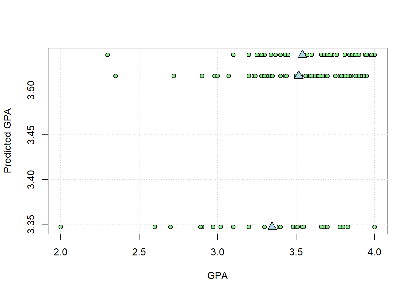
22.2 Statistical Significance
For ANOVA, we think of statistical significance as determining if there is more variability across the three means than is expected by chance (based on the variability within means). For regression, we think of statistical significance as whether we can justify having three parameters to fit the data instead of one. With regression we can test for significance by comparing how good our complete model with three parameter fits compared to a restricted model that predicts all GPAs are the same (the grand mean). Recall from the ANOVA is just regression chapter that this turns out to be an F-test, with SS, MS, df, and p-values equal to those from the traditionally calculated ANOVA.
In R, we can conduct this test by passing the output of the model into the ‘anova’ function. In the ANOVA is just regression chapter we passed in the results from this ‘full’ model and a restricted model. If we send in only one model result the restricted model is implied and run as a comparison:
## Analysis of Variance Table
##
## Response: GPA_UW
##            Df  Sum Sq Mean Sq F value  Pr(>F)
## sit         2  0.8155 0.40774  3.4476 0.03444 *
## Residuals 146 17.2671 0.11827
## ---
## Signif. codes:  0 '***' 0.001 '**' 0.01 '*' 0.05 '.' 0.1 ' ' 1
The table should look familiar. It should match the values done with the standard one-factor ANOVA.
In the plot above, the spread of the points horizontally around the means should be equal to \(SS_{within}\). Let’s check:
## [1] 17.26707This matches the SS for ‘Residuals’ in the ANOVA table, which is \(SS_{within}\)
22.3 Two factor balanced ANOVA example
Next we’ll revisit the data on the effects of Beer and Caffeine on reaction times that we analyzed in the Two Factor ANOVA chapter. This chunk loads in the data and orders the levels.
RTdata <- read.csv("http://www.courses.washington.edu/psy524a/datasets/BeerCaffeineANOVA2.csv")
RTdata$beer <- factor(RTdata$beer,levels = c('no beer','beer'))
RTdata$caffeine <- factor(RTdata$caffeine,levels = c('no caffeine','caffeine'))| Responsetime | caffeine | beer |
|---|---|---|
| 2.24 | no caffeine | no beer |
| 1.62 | no caffeine | no beer |
| 1.48 | no caffeine | no beer |
| 1.70 | no caffeine | no beer |
| 1.06 | no caffeine | no beer |
| 1.39 | no caffeine | no beer |
| 2.69 | no caffeine | no beer |
| 0.28 | no caffeine | no beer |
| 2.24 | no caffeine | no beer |
| 1.15 | no caffeine | no beer |
| 1.53 | no caffeine | no beer |
| 2.43 | no caffeine | no beer |
| 1.71 | no caffeine | beer |
| 2.19 | no caffeine | beer |
| 2.27 | no caffeine | beer |
| 2.35 | no caffeine | beer |
| 2.47 | no caffeine | beer |
| 2.07 | no caffeine | beer |
| 2.56 | no caffeine | beer |
| 2.35 | no caffeine | beer |
| 1.50 | no caffeine | beer |
| 2.63 | no caffeine | beer |
| 2.48 | no caffeine | beer |
| 1.94 | no caffeine | beer |
| 0.62 | caffeine | no beer |
| 1.72 | caffeine | no beer |
| 1.75 | caffeine | no beer |
| 1.84 | caffeine | no beer |
| 1.30 | caffeine | no beer |
| 1.52 | caffeine | no beer |
| 1.31 | caffeine | no beer |
| 1.63 | caffeine | no beer |
| 1.91 | caffeine | no beer |
| 1.33 | caffeine | no beer |
| 0.84 | caffeine | no beer |
| 0.45 | caffeine | no beer |
| 2.05 | caffeine | beer |
| 1.51 | caffeine | beer |
| 1.65 | caffeine | beer |
| 2.68 | caffeine | beer |
| 2.06 | caffeine | beer |
| 1.80 | caffeine | beer |
| 2.68 | caffeine | beer |
| 1.93 | caffeine | beer |
| 1.29 | caffeine | beer |
| 1.93 | caffeine | beer |
| 1.35 | caffeine | beer |
| 1.37 | caffeine | beer |
This data is ‘balanced’, meaning that there are the same number of observations in each cell. You can see this using R’s ‘table’ function:
##
##               no beer beer
##   no caffeine      12   12
##   caffeine         12   12
With a balanced data set, the results from a linear regression analysis will be the same as for the traditional ANOVA. Here’s the result using R’s lm function:
## Analysis of Variance Table
##
## Response: Responsetime
##               Df  Sum Sq Mean Sq F value   Pr(>F)
## caffeine       1  1.2708  1.2708  4.9498 0.031269 *
## beer           1  3.4080  3.4080 13.2748 0.000706 ***
## caffeine:beer  1  0.0083  0.0083  0.0322 0.858395
## Residuals     44 11.2960  0.2567
## ---
## Signif. codes:  0 '***' 0.001 '**' 0.01 '*' 0.05 '.' 0.1 ' ' 1
The model, Responsetime ~ caffeine*beer is telling lm to predict the dependent variable, ‘Responsetime’, by the nominal scale independent factors ‘caffeine’ and ‘beer’ and their interaction.
22.4 Two factor unbalanced design
This next example will use the survey data to study the effects of gender and math preference on students’ predicted score in the first exam. The two (nominal scale) independent measures are ‘gender’ and ‘math’, and the ratio scale dependent measure is ‘Exam1’. This is an unbalanced data set because there are unequal numbers of students that fall into the categories of math preference and gender. We can see that with another table:
##
##         A fair amount Just a little Not at all Very much
##   Man               7            14          5         3
##   Woman            25            62         33         2
You may have been taught that we can’t use a two-factor ANOVA with an unbalanced design like this. But linear regression allows for it
## Analysis of Variance Table
##
## Response: Exam1
##              Df Sum Sq Mean Sq F value  Pr(>F)
## math          3  571.7 190.569  3.0736 0.02974 *
## gender        1   41.8  41.769  0.6737 0.41314
## math:gender   3  350.2 116.721  1.8825 0.13520
## Residuals   143 8866.4  62.003
## ---
## Signif. codes:  0 '***' 0.001 '**' 0.01 '*' 0.05 '.' 0.1 ' ' 1
But here’s where things get complicated. With an unbalanced design you’ll find that the results are different if we switch the order of the independent variables:
## Analysis of Variance Table
##
## Response: Exam1
##              Df Sum Sq Mean Sq F value  Pr(>F)
## gender        1  103.5 103.473  1.6688 0.19850
## math          3  510.0 170.001  2.7418 0.04549 *
## gender:math   3  350.2 116.721  1.8825 0.13520
## Residuals   143 8866.4  62.003
## ---
## Signif. codes:  0 '***' 0.001 '**' 0.01 '*' 0.05 '.' 0.1 ' ' 1
What’s the deal here? It shouldn’t matter which order you state your independent variables. This is true for a balanced data set (try it for the beer and caffeine example above). But for unbalanced designs it can matter. The reason has to do with the columns of the design matrix generated by lm. For a balanced design, the columns - or regressors - are mutually orthogonal, so that each column is pulling out independent sources of variability in our dependent variable. But for an unbalanced design, the columns are no longer orthogonal, so the order matters.
It might help to consider the case of predicting student’s heights from parent’s heights. Suppose we use both mother’s and father’s heights as regressors. There is a strong correlation between mother’s and father’s heights. So if we use mother’s heights as the first factor, there isn’t much remaining variability in student’s height left for the father’s heights to account for. But if we use father’s heigths first, then there’s not much variability left for the mother’s heights to predict. So the order matters:
## Analysis of Variance Table
##
## Response: height
##            Df  Sum Sq Mean Sq F value    Pr(>F)
## mheight     1  184.14 184.137  20.406 1.326e-05 ***
## pheight     1  256.28 256.279  28.401 3.883e-07 ***
## Residuals 139 1254.27   9.024
## ---
## Signif. codes: 0 '***' 0.001 '**' 0.01 '*' 0.05 '.' 0.1 ' ' 1## Analysis of Variance Table
##
## Response: height
## Df Sum Sq Mean Sq F value Pr(>F)
## pheight 1 368.44 368.44 40.8308 2.334e-09 ***
## mheight 1 71.98 71.98 7.9769 0.005435 **
## Residuals 139 1254.27 9.02
## ---
## Signif. codes: 0 '***' 0.001 '**' 0.01 '*' 0.05 '.' 0.1 ' ' 1For an unbalanced anova, the regressors are also not orthogonal, so the order matters. I’ve found a useful discussion on this topic on (stack exchange)[https://stats.stackexchange.com/questions/552702/multifactor-anova-what-is-the-connection-between-sample-size-and-orthogonality]
It turns out that there three ways to deal with this issue with ANOVA. They are called Type I, II and III ANOVAs.
Notice that the SS, df, and MS for the ‘Residuals’ are the same (which serve as the denominator for the F test), regardless of the order. Thus, the fit of the complete model is the same, regardless of the order of factors. The difference is in the way SS is calculated for the main effects. The ‘anova’ function runs a type I ANOVA, and with type I ANOVAs the order of variables does make a difference.
22.5 Type I ANOVA
Remember from the ANOVA is just regression chapter that with regression, the numerator of the F statistic is based on comparing a ‘complete’ model to a ‘restricted’ model. For type I ANOVAs, the SS for the numerator has to do with the order in which the model is increased with complexity. For the current example, consider the fit of the model in the following increasing levels of complexity. Note, the first model, ‘Exam1 ~ 1’, is a fit of a single parameter to the whole data set - leading to a calculation of the grand mean.
a <- lm(Exam1 ~ 1, data = survey)
b <- lm(Exam1 ~ math, data = survey)
c <- lm(Exam1 ~ gender + math, data = survey)
d <- lm(Exam1 ~ gender * math, data = survey)
The function ‘deviance’ takes in the output of ‘lm’ and gives you the sums of squared error for that model. For example, the sums of squared for the simplest model, model ‘a’ is:
## [1] 9830.04This is \(SS_{total}\) The SS for the second model, with just the ‘math’ factor is:
## [1] 9258.333It’s smaller because it’s a more complicated model. Let’s look at how the SS decreases as we increase the complexity of the model in the order chosen above:
## [1] 571.7068## [1] 41.76925## [1] 350.1624These numbers match the values in the ‘Sum Sq’ column when we ran the lm with math followed by gender. Thus the numerators for the type I ANOVA are based on adding each factor (and their interactions) sequentially. This is why type I ANOVAs are sometimes called ‘sequential’. With a Type I ANOVA, putting math as the first factor tests the main effect of math first, followed by tghe main effect of gender, followed by their interaction. This is different than putting gender first followed by math.
This dependence on the order of factors is generally not a desirable thing. That’s why Type II (and then type III) ANOVAs have been developed.
22.6 Type II ANOVA
The easiest way to esolve this problem is to run type I ANOVAs using all combinations of orders and then pulling out the SS that’s most appropriate for the test we want to make. In the example above, the main effect of gender is best studied by comparing gender+math to math alone. So we should pull the SS from the lm fit with math first followed by gender. Conversely, the main effect of math should be pulled from the fit of gender first followed by math. That is, you should use the SS for your factor when it is added last to the list - after the other factors.
To run a type II ANOVA, we need to use the “car” package and use the ‘Anova’ function. Yes, the same name as ‘anova’, but with a capital ‘A’. Welcome to the world of open source software.
Here’s how to use ‘Anova’ to obtain result of the two-factor for gender and Exam 1 using a type II analysis:
## Anova Table (Type II tests)
##
## Response: Exam1
##             Sum Sq  Df F value  Pr(>F)
## math         510.0   3  2.7418 0.04549 *
## gender        41.8   1  0.6737 0.41314
## math:gender  350.2   3  1.8825 0.13520
## Residuals   8866.4 143
## ---
## Signif. codes:  0 '***' 0.001 '**' 0.01 '*' 0.05 '.' 0.1 ' ' 1
This is exactly the same as using lm4.out, which had gender first:
## Anova Table (Type II tests)
##
## Response: Exam1
##             Sum Sq  Df F value  Pr(>F)
## gender        41.8   1  0.6737 0.41314
## math         510.0   3  2.7418 0.04549 *
## gender:math  350.2   3  1.8825 0.13520
## Residuals   8866.4 143
## ---
## Signif. codes:  0 '***' 0.001 '**' 0.01 '*' 0.05 '.' 0.1 ' ' 1
Which is a good thing.
22.7 Type III ANOVA
Type II ANOVA tests for a main effect after the other main effect(s), but what about an interaction? Type III ANOVAs test for a main effect for a factor after accounting for other main effecs AND their interactions. Like type II ANOVAs, the order of the factors doesn’t matter.
For a balanced design, the results of a type III anova will match those from a traditional ANOVA. For unbalanced designs, I often get errors running type III analysis. It happens with this regression example. You can try it for yourself.