Chapter 12 Plotting Distributions of Samples

In this chapter we’ll explore various ways of representing the distribution of scores within and across groups. We’ll be using the survey data and compare the distribution of student’s preferred outdoor temperature grouped by how much they say weather affects their mood. We’ll be plotting graphs summarizing data in variety of ways, pointing out the strengths and weaknesses of each. Note: I stole some of this material from a post by Eamon Caddingan’s page titled ‘Violin plots are great’

As usual, we’ll first load in the survey data:

rm(list = ls())

survey <-read.csv("http://www.courses.washington.edu/psy315/datasets/Psych315W21survey.csv",na.strings = "")

Note that preferred temperature (‘temperature’) is a continuous variable, while the response to the question ‘How does weather affect your mood?’ (‘weather’) is a nominal scale variable or what R calls a ‘factor’. So we can think about ‘temperature’ grouped by ‘weather’.

Before we make any plots, let’s first look at some summary statistics by calculating the mean, standard deviation and standard error of the mean for ‘temperature’ grouped by ‘weather’.

First, we’ll generate a data frame called ‘subsurvey’ by pulling out the relevant subset of the data and removing the NA’s.

subsurvey <- survey[c("weather",'temperature')] 
subsurvey <- subset(subsurvey,!is.na(weather) & !is.na(temperature))

By the way, there is a way to combine the above two lines into a single line using the ‘pipe’ command (‘%>%’). What %>% does is take the output of the thing on the left and passes it in as the first argument to the thing on the right. Some think of the ‘pipe’ as a more elegant way to write code since replacing the same variable in subsequent lines is a bit ugly. Here’s how you do the same thing above in a single line.

subsurvey <- survey[c("weather",'temperature')] %>% subset(!is.na(weather) & !is.na(temperature))

Next we’ll put the levels of the factor ‘weather’ in a sensible order, since R orders things alphabetically by default. Once we’ve done this, all graphs and tables will have the levels in the new order.

subsurvey$weather <- factor(subsurvey$weather,levels= c("Not at all",
                                                        "Just a little",
                                                        "A fair amount",
                                                        "Very much"))

Let’s now calculate some summary statistics (means, sample sizes, standard deviations, standard error of the means, and 95% confidence intervals) for the preferred temperature for each level of the factor ‘weather’. We’ll do this using the R’s summarySE function from the Rmisc package. It’s straightforward. the first argument after the name of the data is the name of the ‘measure’ which is ‘temperature’ and the second argument is the grouping variable which is ‘weather’:

summary <- summarySE(subsurvey,"temperature","weather")

We’ll use the ‘kable’ function in the ‘knitr’ library to present a nice looking table in Markdown. Setting digits = 2 rounds all values to two decimal places.

kable(summary, digits =2)

weather	N	temperature	sd	se	ci
Not at all	12	69.13	7.99	2.31	5.07
Just a little	35	69.53	9.03	1.53	3.10
A fair amount	63	70.98	6.49	0.82	1.63
Very much	40	73.62	6.18	0.98	1.98

You can see in the table that there is a difference in the mean preferred temperature across the groups. Later we’ll use an ‘ANOVA’ to determine if these differences are statistically significant.

12.1 Plotting every point

The most complete way to show the distribution of preferred temperature is to plot every observation as a data point. ‘geom_point’ will to this as a part of ‘ggplot’. ‘geom_point’ allows you to jitter the data points a little along the x-axis so that they spread out a bit. It’s a little weird to deliberately add randomness to your data in the process of visualization, but it works. Keep in mind that your plot will look a little different every time you run it since ‘jitter’ is using the random number generator (though you can fix that with the set.seed function) You can even jitter the ‘height’ of your data along the depend-variable y-axis, which is really weird and wrong, so don’t do that.

ggplot(subsurvey, aes(x = factor(weather), y = temperature, color = factor(weather))) + 
  geom_point(aes(y = temperature, color = factor(weather)), 
             position = position_jitter(width = 0.25, height = 0.0),
             alpha = .8) +
  theme(legend.position = "none") +
  xlab('How much does weather affect your mood?') +
  ylab('Preferred Outdoor Temperature (F)') + 
  theme_bw()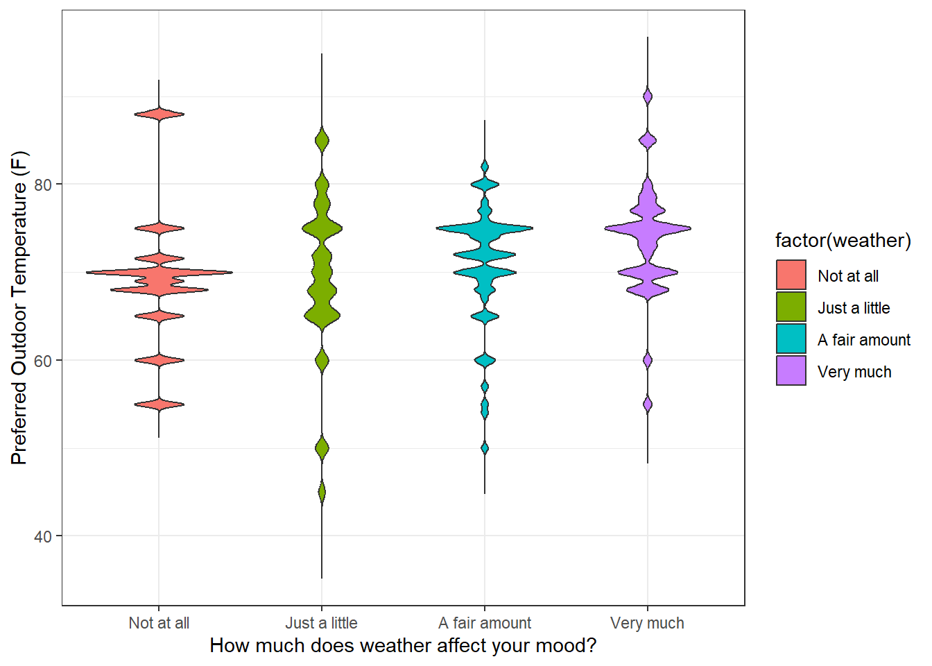

The advantage of plotting every point is that you can see the whole data set. But this can also be a disadvantage. It forces you to rely on your visual system to generate its own estimates of central tendency and variability. And vision is full of biases and illusions - there is a whole subfield of vision research called ‘ensamble perception’ dedicated to this process.

12.2 Violin Plots

Instead of showing very data point, you can generate a ‘violin plot’, which draws a smooth curve representing the frequency distribution of the data. The smooth curves can sort of look like violins, I guess. It’s easy to do this in R:

ggplot(subsurvey, aes(x = factor(weather), y = temperature, fill = factor(weather))) + 
  geom_violin() +
  theme(legend.position = "none") +
  xlab('How much does weather affect your mood?') +
  ylab('Preferred Outdoor Temperature (F)') + 
  theme_bw()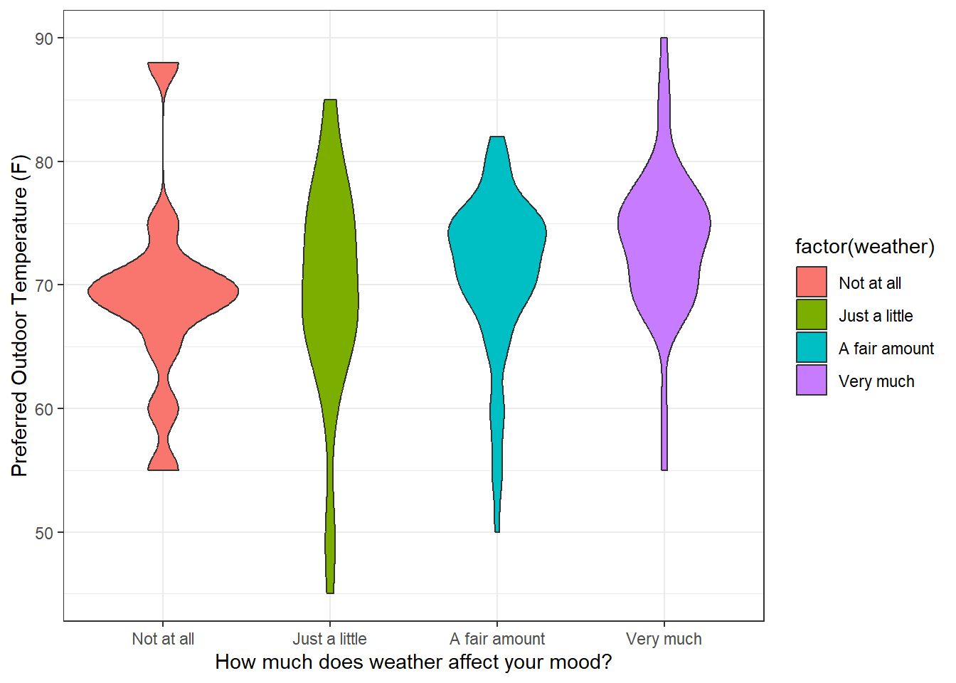

Violin plots are becoming a popular way of summarizing the frequency distribution of data. The eye can more easily estimate the center and spread of the data. One problem with violin plots is that since they represent a discrete distribution with a smooth curve, they can sometimes be a little misleading. For example outliers seen in the individual data plot show up as blobs in the violin plot, as though there were a clump of data points there instead of one.

Also you have to be careful about how R decides to smooth and trim the data. By default, R trims the outliers. If you turn that off, things can look a little different, which is a little scary:

ggplot(subsurvey, aes(x = factor(weather), y = temperature, fill = factor(weather))) + 
  geom_violin(trim = FALSE)+
  theme(legend.position = "none") +
  xlab('How much does weather affect your mood?') +
  ylab('Preferred Outdoor Temperature (F)') + 
  theme_bw()

And there’s a variable ‘adjust’ which determines how much smoothing is used to generate the curves. This can also affect the way things look (the default is ‘adjust’ = 1).

ggplot(subsurvey, aes(x = factor(weather), y = temperature, fill = factor(weather))) + 
  geom_violin(adjust = .2, trim = FALSE) +
  theme(legend.position = "none") +
  xlab('How much does weather affect your mood?') +
  ylab('Preferred Outdoor Temperature (F)') + 
  theme_bw()

This is a little like fiddling with the class intervals in a histogram to make things look the way you want. So there is definitely an element of subjectivity in your choice of parameters when making a violin plot.

12.3 Box and Whisker Plots

An older way to represent the center and spread of a distribution is the box and whisker plot - or sometimes just called a ‘boxplot’.

ggplot(subsurvey, aes(x = factor(weather), y = temperature, fill = factor(weather))) + 
  geom_boxplot() +
  theme(legend.position = "none") +
  xlab('How much does weather affect your mood?') +
  ylab('Preferred Outdoor Temperature (F)') + 
  theme_bw()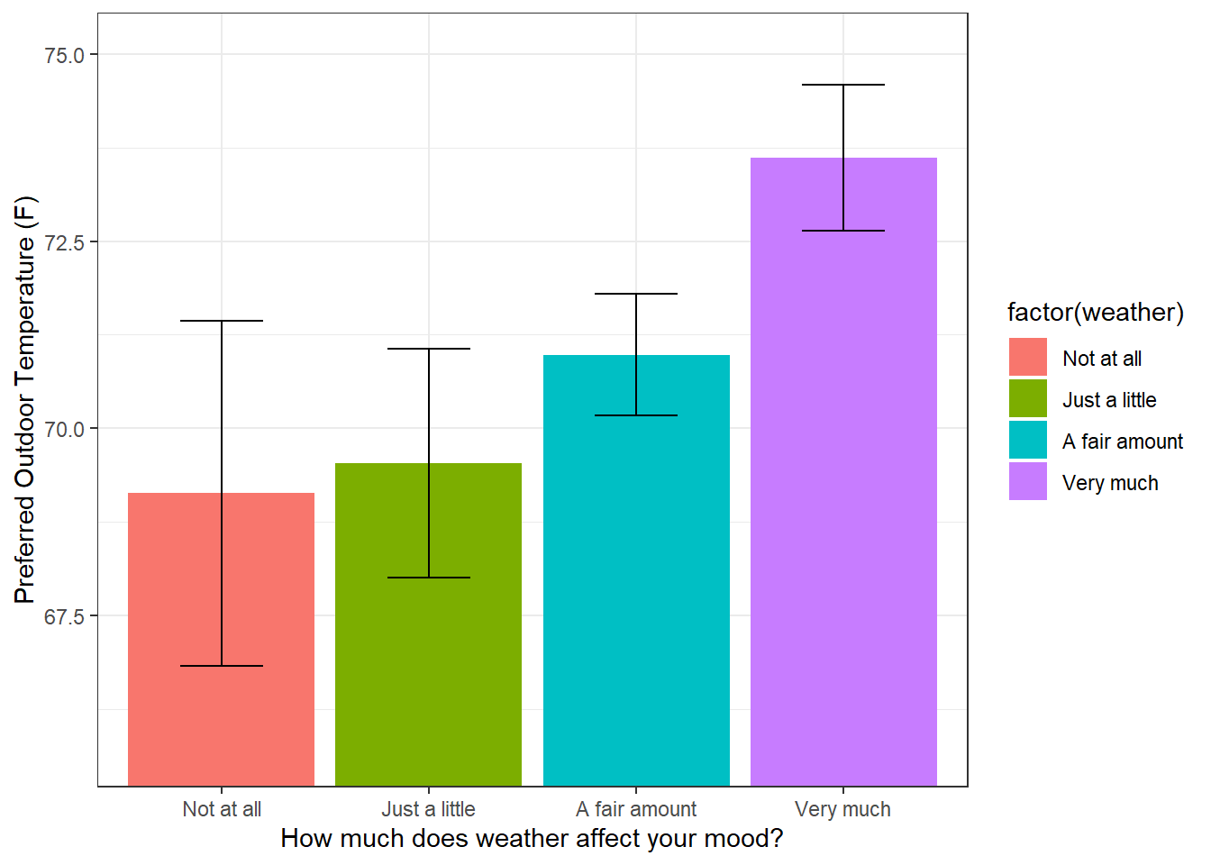

The range of the box is from the 25th to the 75th percentile (\(Q_1\) and \(Q_3\)), and the horizontal line is the median. So the box covers the middle 50% of the distribution. By default, the vertical line (the ‘whisker’) extends from \(Q_1\) minus 1.5 times the interquartile range (IQR, or \(Q_3 - Q_1\)) to \(Q_3\) plus 1.5 times IQR.

The idea behind this to think about what the whisker length means in terms of a normal distribution. For a normal distribution, \(Q_1\) is about 0.675 standard deviations below the mean (qnorm(.25)). The IQR is therefore double that, or about 1.35 standard deviations. Subtracting 1.5 times the IQR from \(Q_1\) leaves you -.67 - 1.5*1.35 = -2.695 standard deviations below the mean. Similarly, the upper end of the whisker will be 2.695 standard deviations above the mean. So the whiskers cover the middle 99.3 % of the normal distribution.

The remaining dots are individual data points that lie outside the whisker. Since these are outside the 99.3% confidence interval for a normal distribution, you can consider then as outliers.

12.4 Bar graphs with confidence intervals

The simplest, and most impoverished plot is a bar graph of the means with error bars representing confidence intervals based on a normal distribution. Do do this with ggplot you need to plot both the bar and the error bars in succession. A typical plot, like the one below, will have 95% confidence intervals, which corresponds to error bars \(\pm\) two standard deviations from the mean. I’ve also added the plots of the individual data points to you can see how well the confidence intervals represent the data

ggplot(summary, aes(x = factor(weather), y = temperature, fill = factor(weather))) +  
  geom_bar(aes(fill = factor(weather)), stat = "identity") + 
  geom_errorbar(aes(y = temperature, ymin = temperature-2*sd, ymax = temperature+2*sd), 
                color = "black", width = 0.4) + 
  geom_point(data = subsurvey,aes(x = factor(weather), y = temperature), 
             position = position_jitter(width = 0.25, height = 0.0),
             alpha = .5) +
  theme(legend.position = "none") +
  xlab('How much does weather affect your mood?') +
  ylab('Preferred Outdoor Temperature (F)') + 
  theme_bw()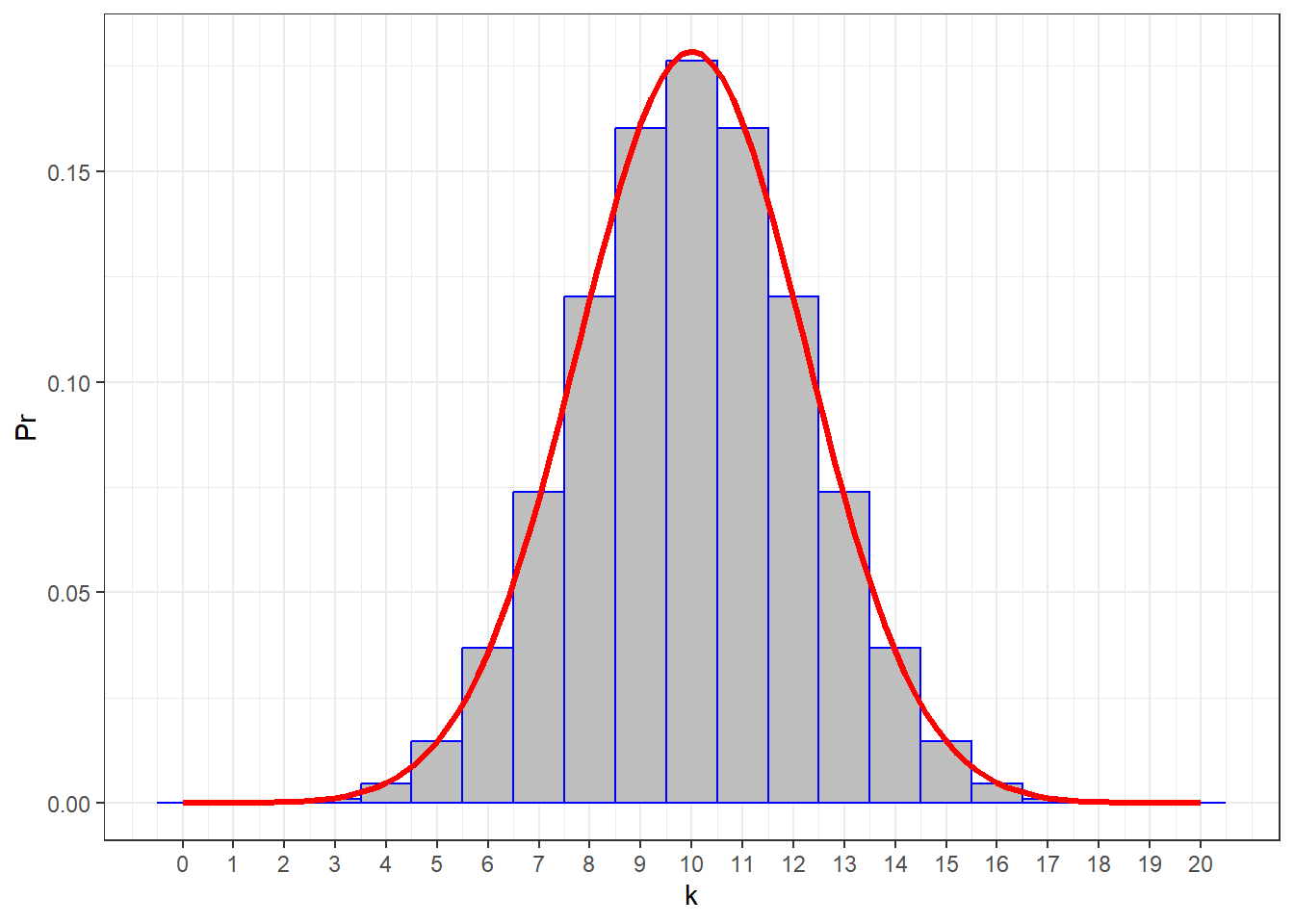

Bar plots with error bars are criticized because they aren’t appropriate for non-normal and especially skewed data, since the confidence intervals are equally spaced above and below the mean. For this reason, the field has been gradually moving toward the previous options like the violin plot.

Notice how these plots so far are successful, to varying degrees, at illustrating the distribution of individual data points within the level of each factor. These plots are not, however, good at visualizing the differences in the means across levels. For this, we need to think not about standard deviations of the samples, but about standard errors of the mean.

12.5 Bar graph with standard errors

The most common plot for representing differences betweeen means is the bar graph with error bars representing the standard errors of the mean. For this plot, I’ve re scaled the y-axis to focus in on the range covering the error bars, which does not necessarily include zero.

ylimit <-  c(min(summary$temperature-1.5*summary$se),
             max(summary$temperature+1.5*summary$se))

ggplot(summary, aes(x = factor(weather), y = temperature, fill = factor(weather))) +  
  geom_bar(aes(fill = factor(weather)), stat = "identity") + 
  geom_errorbar(aes(y = temperature, ymin = temperature-se, ymax = temperature+se), 
                color = "black", width = 0.4) + 
  theme(legend.position = "none") +
  coord_cartesian(ylim=ylimit) + 
  xlab('How much does weather affect your mood?') +
  ylab('Preferred Outdoor Temperature (F)') + 
  theme_bw()

Keep in mind that the error bars are standard errors - not standard deviations. Remember, the standard error is the standard deviation of the distribution of means expected from a sample of this size. So these error bars serve to visualize how different the means are from each other in terms of running multiple experiments. We discussed earlier how out that for two means, if the error bars overlap then you can be pretty sure that a t-test will result in a p-value greater than 0.05. That is, you need a bit of a gap between the error bars to reach statistical significance. In the plot above, do you think a comparison of any of the two means would be statistically significant?

A final plot is with error bars representing 95% confidence intervals for the distribution of means. These are calculated the same way that we did in the chapter Confidence Intervals and Effect Size. The summarySE function returns these confidence intervals in the ci field. So all we need to do is replace the se above with ci:

ylimit <-  c(min(summary$temperature-1.5*summary$ci),
             max(summary$temperature+1.5*summary$ci))

ggplot(summary, aes(x = factor(weather), y = temperature, fill = factor(weather))) +  
  geom_bar(aes(fill = factor(weather)), stat = "identity") + 
  geom_errorbar(aes(y = temperature, ymin = temperature-ci, ymax = temperature+ci), 
                color = "black", width = 0.4) + 
  theme(legend.position = "none") +
  coord_cartesian(ylim=ylimit) + 
  xlab('How much does weather affect your mood?') +
  ylab('Preferred Outdoor Temperature (F)') + 
  theme_bw()

Bar plots with standard errors and 95% confidence intervals have been much maligned recently, but I’ll try to make a case for them. First, they criticized because the error bars are small compared to the data. But remember, these plots are not designed to represent the distribution of the individual samples - but rather the sampling distribution of the mean. So they serve a different purpose than violin or boxplots. Second, these plots are criticized because they are not appropriate if the samples are not normally distributed. However, this is a common confusion. Remember, we are representing the distribution of means, and as you recall, thanks to the Central Limit Theorem, we can be reasonably confident that the distribution of means will be pretty much normally distributed even if the population that the samples came from is not.

So in summary, yes, bar graphs with error bars as standard deviations are problematic, but bar graphs with standard errors of the means are a good way of representing differences between means.